Please Note: This article is written for users of the following Microsoft Excel versions: 2007 and 2010. If you are using an earlier version (Excel 2003 or earlier), this tip may not work for you. For a version of this tip written specifically for earlier versions of Excel, click here: Displaying Images based on a Result.
Dave has a large database that he keeps in an Excel workbook. It consists of material samples, and he uses the VLOOKUP function to generate various forms and reports. Dave wants to include a bitmap image on the form that changes according to one of the variables. For instance, if the form is describing an apple, then Dave wants a picture of an apple to appear; if describing a pear, then a pear should appear; and so on.
This is certainly a challenging task, but it is one that can surprisingly be done without macros. The steps are involved, but not that difficult to perform once you get to it:
=IF(G1=1,"apple",IF(G1=2,"pear",IF(G1=3,"orange","")))
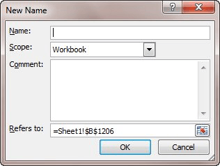
Figure 1. The New Name dialog box.
=INDIRECT(Sheet1!$A$1)
Now, whenever the fruit name in cell A1 changes (which is, in turn, based on the value in cell G1), the image will change.
ExcelTips is your source for cost-effective Microsoft Excel training. This tip (10450) applies to Microsoft Excel 2007 and 2010. You can find a version of this tip for the older menu interface of Excel here: Displaying Images based on a Result.

Create Custom Apps with VBA! Discover how to extend the capabilities of Office 365 applications with VBA programming. Written in clear terms and understandable language, the book includes systematic tutorials and contains both intermediate and advanced content for experienced VB developers. Designed to be comprehensive, the book addresses not just one Office application, but the entire Office suite. Check out Mastering VBA for Microsoft Office 365 today!
The graphics you place in a worksheet can do more than just look pretty. You can also assign macros to a graphic, which ...
Discover MoreIf you want to create a line in your worksheet that is a specific length and slope, there are a couple of ways you can do ...
Discover MoreYou can add all sorts of objects to your workbooks, including video clips. Here's the pros and cons (along with the ...
Discover MoreFREE SERVICE: Get tips like this every week in ExcelTips, a free productivity newsletter. Enter your address and click "Subscribe."
2021-09-24 16:20:05
Ronmio
One of the best tips yet.
2020-02-14 13:01:32
Roberto
Very nice instruction, thanks.
Kameswaran the issue with the reference is that if you leave the cell with the number blank it does not work.
Put a number there (G1)
2019-08-13 17:56:19
Peter Atherton
Kat,
I'm not sure how the Name cell is greyed out but there is another way.
Select B4 --> Click Formulas Tab --> Defined Names Group --> New
In the New Name form type your name in the Name text Box, in the Refers to textbox check that the cell is the right one and click OK
If the refers to cell is wrong, click the Up arrow on the right of the textbox to return to the sheet and select the right one and press enter and then clicl OK button.
(see Figure 1 below)
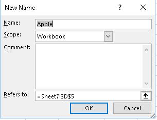
Figure 1.
2019-08-12 09:48:46
Kat
I'm having trouble with step 2, "Enter the name "apple" into the Name box, to the left of the Formula bar. This defines the name "apple" to refer to cell B4." It is greyed out and will not allow me to type into it. I have clicked, double clicked, made sure B4 was highlighted, tried the different tabs at the top, etc. I can not type into the name box. How do I do that?
Thank you,
Kat >^..^<
2019-08-08 06:29:44
Rm
Hi Allen,
Thanks for your sharing of the great tips.
I have an excel file which is inserted an image object with "link to file", when I replace the image, it reflects to the excel, that works fine, but once I copy the excel and image files in new folder, the path of the object is still linked to old path, is that anyway it could be a relative path instead of absolute path in this case? (without VBA/ Marco)
Thanks!
Rm
2019-04-23 08:08:54
Elvis
Discovered you don't need to insert the pictures to be displayed as objects, you only need to do this for the one serving as a placeholder for them, so that you can attach a formula to it.
Still looking for solutions for the auto-update when image selected is changed.
2019-04-23 07:09:13
Elvis
Tried the revised steps of inserting the pictures as objects on the Excel 2007, I'm able to select the picture object in the last step & edit the formula to =Picture, however, when the values change, the picture displayed doesn't get updated.
If the image is selected, and the =Picture formula is reentered, then the picture updates to the next one selected.
Pls, what can be done to make this auto update?
I've checked my calculations settings - it's on auto update
2019-04-23 06:05:56
Elvis
Tried this on Excel 2007, but the last step couldn't be done. After selecting the image, entries into the formula bar are disabled. Couldn't continue thereafter.
2019-04-10 12:28:50
Andy
Thank you, your steps helped me earn much glory in my office
2018-05-26 04:51:52
Keith
Hi
I am using Excel 2016, would this be an issue?
I have followed the steps but without any success.
Is there any chance of a sample file to see how it is set up?
Thanks in advance.
2018-05-25 14:51:11
Pat J
Any Chance of getting a sample file, getting confused as to which sheet to put the formulas on :(
2018-03-07 15:09:52
Kelton Collopy
I am also using a MAC, I read the comments and watched the video but I don't have the same tools for Name Manager as the video or to define New Nam as described above. Thanks
2018-03-07 14:39:29
Kelton Collopy
How does this work in versions of Excel beyond 2007 and 2010? I don't get New Name dialog box shown when clicking Define Name, I simply get Define Name dialog box.
2018-02-06 12:35:04
Gary
None of the comments and fixes work for Office 365. Always says unable to assign reference.
2017-08-03 12:13:20
Paul
Hi,
This way works but for what I need to do, i'd need to define a number to 50-60 items. Is there a way to include an IF, or INDEX instead of using =Picture when selecting the image?
Paul
2017-05-05 10:49:43
Slawek
Thank you for the tip but it seems to work for one line, what we have 100 rows with three types of pictures (I need it to show the trend increasing, stable, decreasing the up to 200 risks with individualized icons showing on of 3 possiblities of trends. Does that mean I have to define "name" for each line? It would be not production. Do you think there is a way to parametrize this?
2017-03-17 05:42:55
Kameswaran
Displaying Images based on a Result is not working for me Sir. Can you share sample sheet. Thanks in Advance
2017-01-26 13:07:37
JimD
Woops ... minor correction to prior post about linked file images. After further testing, it appears that changing the path+file's name or extension does not actually do anything ... the original image loaded remains unchanged. I tried doing Data > EditLinks > Update but it did not seem to help.
All other instructions in prior two posts are fine.
2017-01-26 12:13:55
JimD
OK y'all are going to LOVE this. My prior rewrite of the instructions (post just after this) is correct. But you can, if you wish, store the "library" of "fruit" picture objects as EXTERNAL LINKS to filename.bmp pictures on your hard drive ... I haven't checked but this should reduce the xls size bigtime if you have a lot of pics ... AND it allows you to change the source-picture just by saving a new copy of the picture in the hard drive folder. I am using this to create a Pictorial Directory of the GwinnettSymphonyChorus ... lots of pictures, and some folks never seem to be satisfied with the first try at their ugly mugs. But, I digress ...
To accomplish this,
A. Save the picture in the folder as a BMP file ... this is essential ... PNG, etc will not work (for the initial insert).
B. Modify Step#3 in the post below to:
Insert > Object > Create From File > (Check Link to File but not Display as icon) > Browse to the BMP file you want to use and click OK.
... That's all there is to it.
Interesting followup note: Once you get that all done, and examine the formula assigned to the picture-object, you'll see:
=Paint.Picture|xxxxxxx
where xxxxxx is the full path+filename to the picture (.BMP) you chose.
AT THIS POINT (after the BMP is properly connected to the cell), I found by experimentation that I could edit that formula and just change the extension to .PNG (I had a PNG version of the same person's "new" picture in the folder) ... and it updated the pic linked into the sheet just fine.
The advantage of using PNG's rather than BMP's is mainly that PNG's are MUCH smaller files than BMP's. I haven't tried it but I presume this would work for .JPG files as well ...
Just remember: the initial cell needs to be populated by a BMP, whether it is a Bitmap Image from Paint, or an external file. Enjoy!
2017-01-26 11:49:14
JimD
OK ... combining several of the prior suggestions (the real key is NOT to Insert > Picture but rather to Insert > Object > Bitmap image ... so that the final Dynamic Image cell can have a formula defined for it) ... here is a complete rewrite of the original instructions - hopefully removing ambiguities. I did this on Excel 2007.
=====================================
1. On a new worksheet, select a cell (such as cell B4).
2. Enter the name "apple" into the Name box, to the left of the Formula bar. This defines the name "apple" to refer to cell B4.
3. With cell B4 still selected, display the Insert tab of the ribbon and use the Object tool to insert a Bitmap Image (don't check "icon") … a Paint edit box opens up > paste the (copied) picture of the apple > close Paint
4. Enlarge the width and height of cell B4 so that the picture of the apple is contained entirely within the cell … manually slide the pic in the cell boundaries to center it if desired.
5. Repeat steps 1 through 4 for each of your other fruit-pictures, placing each picture-object in a different cell and naming them according to the contents of the picture. (For the sake of this example, I'll assume that "pear" is cell D4 and "orange" is cell F4.)
6. On the worksheet that will contain your form, create a formula (this assumes it is put in cell A1) that will contain the names of the fruit, such as the following formula, which displays "apple," "pear," or "orange," depending on the value in cell G1:
=Choose(G1,"apple","pear","orange")
7. It is important that the formula reference the names exactly as you defined them in step 2 for each fruit's picture-objects. For the sake of this example, I'll assume that you entered this formula in cell A1 of Sheet1.
8. Make sure cell A1 is selected and Display the Formulas tab of the ribbon.
9. Click the Define Name tool. Excel displays the New Name dialog box. (See Figure 1.)
10. Replace the contents of the Name box with the word "Picture".
11. Replace the contents of the Refers To box with the following formula:
=INDIRECT(Sheet1!$A$1)
12. Click the OK button. You've now defined the name "Picture" to contain the formula entered in step 10.
13. On the worksheet that will contain your form, select the cell where you want the dynamic image to appear.
14. Repeat steps 3 & 4, putting a "dummy" picture-object (it doesn't matter which one) in this cell where the dynamic image should appear
15. Make sure the picture-object that you inserted in steps 13-14 is selected.
16. In the formula bar, enter the formula =Picture. (This is the name you defined in steps 7 through 12.) The picture should change to reflect whatever fruit is named in cell A1.
Now, whenever the fruit name in cell A1 changes (which is, in turn, based on the value in cell G1), the image will change.
====================================
I hope this solves all future issues.
2017-01-26 10:38:23
JimD
I have Excel 2007. I understand the "intent" of this setup, and have tried these 16 steps in about 6 different minor variations, because step#16 is impossible to do. Step 15 says to SELECT the "dummy" picture ... not the cell that holds it. Step 16 says to type a formula in ... but Excel *does not allow* a formula to be typed in for a picture-object, just for the cell that holds it. Please help!
2017-01-03 09:48:29
Yenit
Perfectly working! Thanks for a cool tip of reducing manual work :)
2016-12-14 02:30:04
Shoaib
Got it working for multiple dynamic images by creating names e.g Picture1 = INDIRECT(Sheet!$A$1), Picture2 = INDIRECT(Sheet!$B$1), Picture3 = INDIRECT(Sheet!$C$1) ... Works fine for me
2016-12-14 01:55:15
Shoaib
This works well for one cell to display the an image dynamically . However, I have about 12 cells that need to dynamic images based on the 12 different values . I cant get this to work .. all help on this is welcome
2016-11-30 15:17:52
David Nunn
I have tried every combination as I reported on 29th of November. I still cannot get past step #10.
I have also tried the video on You-Tube, as suggested by WillB on 18 Dec. 2015. I cannot make that work either. https://www.youtube.com/watch?v=0xJ22YLLy9M
It must be me. I am stuck and need to solve the problem. Help.
2016-11-29 04:33:02
David Nunn
I am stuck on line #10 as I continually get an error message saying a Syntax error. I have copied exactly as you explained, "Picture" and =INDIRECT(Sheet1!$A$1) What am I doing wrong.
Please help.
David.
2016-11-09 16:07:26
jon
This works fine but, if cell A1 is left blank, how can I have the cell for the picture left blank as well.
2016-02-05 13:12:32
Adriana
It works perfectly!! Thanks!
It works for Excel graphs too! The "database" graph must be within a cell, just like the images.
2015-12-18 10:42:48
WillB
I could not get this to work using Excel 2013.
However, this video on Youtube provided simple instructions and I got it to work first try.
https://www.youtube.com/watch?v=0xJ22YLLy9M
2015-12-17 18:44:41
mjwilson
I got it to work but have a slight issue. I've tried VBA and it was glitchy so came to this method.
How I got it to work:
To simplify I skipped a step, but after you get it to work you can see how to modify it to your own needs easily.
Follow instructions up until Step 6. Instead of writing a formula in cell A1 - make that your end result. So type in "apple" no quotes - or whatever it is you named your cell in B4. (The name of the cell shouldn't have quotes either)
Keep following the steps as described not using quotes around anything.
As others described instead of using insert picture in step 14 use insert>object>bitmap image (make sure you don't select display as icon) Hit the OK button, and close down the box that pops up.
The image will already be selected and you'll see a formula already in the formula bar. Change that to the =Picture instead and hit the enter key.
The image will resize to however you have it set.
Now go back to cell A1. Change the text to whatever you named another cell, in the example listed D4 is called Pear, so type that in, no quotation marks. The image doesn't automatically update. This is my problem. However if I click on the image, go back up to the formula bar, and hit enter, the image will update. It's as if I have to activate it every time, instead of it automatically doing it when the cell in A1 changes.
I hope I helped someone and hope I can find a solution too.
2015-07-23 20:21:29
Derek
Thank you for this tip, it works great for my purposes.
One question I have is if it's possbile to have this work on a sheet that is protected. Currently when I have the sheet protected and I change the value that drives which picture is visable, I get an error that I'm trying to update a cell or chart on a protected sheet. I have tried unlocking all the cells the pictures overlap, but that doesn't work.
Is anyone able to get this to work on a protected sheet?
Thanks!
2015-05-01 04:06:57
Richie
A CHOOSE formula will work better than the embedded IF statements. Ie- CHOOSE(G1,"apple","pear","orange")
2015-03-26 03:20:29
lyn
i am trying to have the whole range of picture change but it won't work.
it will work when i only have for one box.
i am figuring that i need to make sure the offset covers the range but can't seems to make it work. please help
2015-03-19 08:13:57
Jonny
Worked perfectly for me thank you for your tip
2015-02-19 08:14:06
Michael
Thank you. This worked perfectly for me. I took some time to read and understand the instructions but it worked first time. In understanding how the formulas worked I was able to rework it to more suit my application. Thank you again I really appreciate the time taken to outline the process.
2015-02-16 10:18:35
Gazza
Shunt, I Found the following works well for displaying an image based on the value of a cell.
If Range("A1").Value = Range("B1").Value Then
ActiveSheet.Shapes.Range(Array("Picture 1")).Visible = msoTrue
Else
ActiveSheet.Shapes.Range(Array("Picture 1")).Visible = msoFalse
End If
2015-02-11 13:47:00
Brian Cummings
Followed the steps exactly but it wouldn't work. Went with the M.Davis method of putting "apple" "apple" quotations around both words and it worked perfectly.
2015-01-27 02:01:47
Ayoub
I guess the instructions could have been worded better, but I finally figured out the the article was trying to communicate and it worked.
So THANKS!!
2015-01-20 08:55:44
Fernando
I tried to insert a picture in step 14 but it didn't worked. Then I tried to insert an object like Denise said and it worked perfectly. Thank you guys!
2015-01-11 06:58:32
John
Hi Matt,
Try the link I suggested (June 2014). It only takes 2 minutes.
Very easy to follow and works a treat, using Index and Match on a table of pictures and names.
2015-01-10 16:53:54
Matt G
I have gone all through the comments using Excel 2013, I have tried Gobinaths Add camera, I have tried Haps Quotes and no Quotes, I have tried moving formulas to Cell $A$1. This simply does not work as written or is too misleading as written to translate into a working instruction. Is it at all possible for someone who got this to work to either detail EXCATLY what steps they went through to get it to work including which Cells they had highlighted at which times, when they did and did not use quotes. Ideally a video would be created that we can just copy click for click. Would love for some assistance
2014-10-10 02:42:57
Meng
Does this actually works on 2010?
2014-09-09 21:02:16
denise
2007 USERS!!
MAKE SURE YOU INSERT OBJECT NOT IMAGE _ OTHERWISE YOU WILL NOT BE ABLE TO WRITE A FORMULA!
2014-08-25 02:09:15
Nugraha
Thank you so much fro this tip! Exactly what I'm looking for.
2014-06-18 05:14:29
John
Charlotte, please try the link I suggested, it works a treat. The images actually 'float' on the spreadsheet and can be moved anywhere.
2014-06-17 09:34:14
charlotte
Ok I give up, I told my boss that I had seen a way of doing this, but he is unimpressed that I have taken all day and got no pictures showing. This would be sooo useful if it would work.
All I get is a 0,(zero) where the picture should be.
The more I read the other comments the more confusing it all gets.
Help please
2014-06-10 14:19:27
John
Couldn't get this to work with Excel 2010 (could be me)but found this a great alternative for inserting up to 5 from 9 hazard pictograms on the records of over 500 different chemicals.
https://www.youtube.com/watch?v=P4XriuikOs8
2014-05-23 07:47:20
MarkA
A little confusing perhaps but after I'd applied myself to it for a while I got it on the third attempt - very good and thanks for this.
2014-03-11 15:38:04
Grace
I entered a # in cell G1 (1,2,3) and used a vlookup to provide the range name, where 1=1st object etc. I changed to Range1, Range3, Range4 to remove the issue with using the word apple.
Works great - thanks to all!
2014-02-12 12:28:48
RJ Simons
When you begin Step 9 you need to be in a blank cell - it doesn't matter which one.
Then define the name "Picture" and enter =indirect(CELL) point to the cell with the if statement
Then your =picture will work.
2014-01-31 14:24:19
Hi,
I followed directions just as Allan articulated and for some reason it won't work. on step 16, once I enter =Picture and press enter, it won't call it but an error message comes up that says:
Reference is not Valid.
please kindly advise.
2014-01-17 15:12:42
Shunt
This worked in Excel 2010. Unfortunately it broke the rest of my VBA code. For those who had the same problem, you might have better luck putting all of the pictures on top of each other and editing their .visible property based on the control cell's value. It may not be the most elegant way, but it worked for me. Here is some of my VBA code to get you started, where B12 is a drop-down and S2:S4 is the list of choices for the drop-down.
Private Sub Worksheet_Change(ByVal Target As Range)
Select Case Target.Address
Case "$B$12"
If Range("$B$12").Value = Range("$S$2").Value Then
Shapes("Picture 17").Visible = True
Else
Shapes("Picture 17").Visible = False
End If
If Range("$B$12").Value = Range("$S$3").Value Then
Shapes("Picture 11").Visible = True
Else
Shapes("Picture 11").Visible = False
End If
If Range("$B$12").Value = Range("$S$4").Value Then
Shapes("Picture 12").Visible = True
Else
Shapes("Picture 12").Visible = False
End If
Case Else
End Select
End Sub
Good luck,
Shunt
2014-01-17 13:30:00
M.Davis
Just tried it with charts and it worked perfectly for me other than when I changed the numbers (from 1 and 2 as options to text):
(eg. =IF(A1=1,"Sales"))
to text such as
=IF(A1="Sales","Sales","")
I had to put quotations marks around the text. Then it worked like a charm. :)
2013-12-11 13:40:47
DippyDoo
Not only did this not work, but after reading the comments and trying to insert a bitmap instead, my excel completely locked. I had to force close excel 2010 from the task manager to do anything else. With the picture selected, (steps 13-16), typing the =Picture into the formula bar does not work for Excel 2010. I receive the error 'reference not valid'. When I start typing the name, excel recognizes it, and I can Tab the rest of it in (as if entering a formula). After going through the name manager (Ctrl + F3) to verify that all the information was correct, I'm still not sure what to do to make it work. I wouldn't consider myself an excel expert, but i'm also not a beginner. Anyone have any ideas?
2013-12-10 14:11:16
neil
It worked for me once I added "Insert Object" (which wasn't in my regular Insert menu) to the Quick Access Toolbar and used it to add a bitmap image as described below.
2013-12-10 12:16:17
Gaz
Yeah, this is an unholy mess isn't it/ Mr Wyatt should perhaps have reviewed and updated this before sending it out today. Step 12 refers to a formula entered in step 10 but should instead refer to step 11. Step 15 refers to the picture inserted in step 13 but should instead say step 14.
It does work, but you have to include the detail that when you're doing steps 8-11 (clicking the formulas tab and defining a name) that you must first go back and make the active cell the one that you've entered your INDIRECT formula in. (cell A1 or whichever you used)
Doing that it works for me in Excel 2010, but with an annoying error. I find that if I enter a number other than 1,2,3 then whatever the last picture shown in the cell was is the picture that remains there. In other words I can 'overwrite' the inserted picture with one of the ones specifically set, but can't overwrite with a null picture. It's as if the final "" in the nested if formula isn't working as it should
2013-12-10 10:03:19
jpeter
I have tried all the "comments" and still could not get this to work. Has anyone been able to resolve? I am using Excel 2010.
2013-12-10 09:21:58
Bryan
I've had mixed luck with this sort of thing, but I think I mostly need more practice. If you don't do it EXACTLY right it has a tendency to fail.
If you have more than 3 pictures and you don't want to have so many nexted IFs (IIRC, you are limited to 64 in xl2007+), you can use CHOOSE instead: =CHOOSE(A1, "apple", "pear", "orange") is functionally the same as Allen's formula. If you set up the tables properly, you could also use INDEX/MATCH to reference the right cell -- and then you can use words to choose the right picture instead of letters.
2013-11-23 12:23:14
Roeland
For step 14, it does matter which picture. Try doing insert -> object -> bitmap. It will open paint, just close it. This gives you a blank image that you can use a formula in. That fixed it for me at least.
2013-11-13 22:06:23
Gary
This is great, working very well. much appreciated.
2013-07-22 07:45:50
jow
I just followed all the steps and it works fine (with bitmap AND with picture). Thanks for the tip!
2013-07-21 04:53:30
qc
I don't think you can select and insert a picture, then use a formula in Excel 2007 (step 16).
What works is if you insert a Bitmap Image (Insert > Object) then use a formula for that bitmap image.
Try it
2013-05-01 10:08:27
jmathane
Thanks for this article. I could complete everything (changing "," by ";" in the IF statement).. until last step. I inserted a picture, selected it.. and I definitively can't enter a formula. I can enter a formula only if a select a cell, not a picture. I use Excel 2007. I guess that there is some 'hidden' way to associate a picture with a formula .. Thanks for your help !
2013-03-27 17:43:16
Mateo
Sorry, correction to my previous....not the very last step. Step "14" - insert the pic again??? Its floating...not part of the cell. Im using 2007. Ive tried everything. Nevermind what Im trying to do with it....I cant get above to work with the instructions given.
2013-03-27 17:14:46
Mateo
Cant get the last step to work in Excel 2007. Clearer instructions would be highly appreciated and/or any help. Keep getting Circular formula errors. Help!
2013-01-02 12:53:39
Hap
Well, everyone this routine works once you understand "how" and "why". First you need to understand how the INDIRECT Function works in Excel. It evaluates a raw text string (i.e. apple not "apple" and returns the value of apple (no quotes) which in this case a picture of an apple in cell B4). By the way, the name of cell B4 is apple. The confusing part is that "apple" is the convention used for a text string in Excel Formulas so it must be typed "apple" to get the formula to work. Unfortunately, if you try to enter the B4 cell name as "apple" Excel 2010 throws up immediately. It doesn't help that Mr. Wyatt tells us in step #2 to enter the name "apple" into the Name Box. This will not work! Then on the other hand he could have been using the quotes to identify the specific word "apple" in instructional writing language. Unfortunately, Excel doesn't want instructional language it wants "Excel Language". He makes the same mistake in step 10 and 12 instruct-ing us to enter the word "Picture" when it should be Picture or "Picture" (without quotes). The ONLY place quotes should be used in this exercise is in the IF formula (i.e. =IF(G1=1,"apple", etc.) If you don't enter the quotes the formula won't work. As a side note I had trouble getting the command =Picture to work so I used the word PictureFormula to name the command then =PictureFormula as the command and it worked (I can't explain why?). Finally, make sure you are in cell A1 (highlighted) when doing step 8 or the formula will not work correctly. Well I hope this helps everyone. I'm sending the exercise in to MENSA to see if they want to use it on their next test. I'm not a MENSA member and if I told you how many hours it took me to figure this out you'd understand why!!! Happy INDIRECTing!
2012-06-27 08:50:05
Rob
Follow Gobinath's instuctions... I got it to work with that...
2012-06-26 20:18:18
Assie
Tried all the above but doesn't work. I really need to find a way to make it work!
2012-04-25 14:34:37
Rob
I still can't this to work in Excel '07. I dont seem to see an "edit picture" fuction. I can paste a picture as a microsoft drawing object, but that still doesnt fix the problem... has anyone else gotten this to work past step 9?
2012-04-16 16:44:20
Gobinath
excel option ->Customize -> commands not in ribbon->Camera->Add->OK
executing the above and try the last step it works . let me know if it doesn't .
2012-02-27 13:05:58
Styx
It works, but not that easy. you have to insert a fake (empty, not white) picture in the cell where you want to have the pictures to appear. How: insert any picture in the cell, RMB, edit picture, convert to Microsoft Office object, and delete content.
select the empty picture and add the text =Picture in the formula bar.
2012-01-05 07:40:21
R.A. Melman
Doesn't seem to work.
I get the same =Picture failure as Raj.
When I choose Insert Object > Bitmap, I can place =Picture in the formula, but still no result.
No picture changing.
2011-11-03 13:33:48
raj
This does not work. In the last step, I am not able to enter formula "=Picture" when the picture is selected.
Got a version of Excel that uses the ribbon interface (Excel 2007 or later)? This site is for you! If you use an earlier version of Excel, visit our ExcelTips site focusing on the menu interface.
FREE SERVICE: Get tips like this every week in ExcelTips, a free productivity newsletter. Enter your address and click "Subscribe."
Copyright © 2026 Sharon Parq Associates, Inc.
 Please Note:
This article is written for users of the following Microsoft Excel versions: 2007 and 2010. If you are using an earlier version (Excel 2003 or earlier), this tip may not work for you. For a version of this tip written specifically for earlier versions of Excel, click here:
Please Note:
This article is written for users of the following Microsoft Excel versions: 2007 and 2010. If you are using an earlier version (Excel 2003 or earlier), this tip may not work for you. For a version of this tip written specifically for earlier versions of Excel, click here:
Comments