Highlighting After-Hours Times

Tom has a worksheet that contains start times and end times for jobs. All times are entered in 24-hour notation. He needs a way to highlight any time that is after 17:00 (5:00 pm) or before 08:00 (8:00 am).

This is precisely the situation in which Conditional Formatting really shines. How you put together the formatting rules, though, depends on how your data is set up and what, exactly, you want to highlight.

Let's say that Tom's data is in columns A and B. In column A he enters a start time and in column B he enters the end time. If Tom wants to highlight only those start times that are in the after-hours range, he could follow these steps:

1. Make sure all the cells in column A are formatted as times. This is important because it means that Excel will evaluate your comparisons in the Conditional Formatting rule properly.
2. Select all the cells in column A that might, at some point, contain a start time. You can, if desired, select all of column A, but that might be overkill.
3. Make sure the Home tab of the ribbon is displayed.
4. Click the Conditional Formatting option in the Styles group. Excel displays a palette of options related to conditional formatting.
5. Choose New Rule. Excel displays the New Formatting Rule dialog box.
6. In the Select a Rule Type list, choose Format Only Cells That Contain. (See Figure 1.)



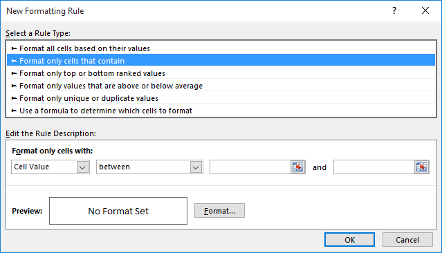
Figure 1. The New Formatting Rule dialog box.

7. Make sure the first drop-down list in the Edit the Rule Description area is "Cell Value." (This should be the default.)
8. Make sure the second drop-down list is "Not Between." Two boxes appear to the right of the drop-down list where you can enter an earlier time and a later time.
9. In the earlier time box, enter 8:00.
10. In the later time box, enter 17:00.
11. Use the format controls to set your highlighting any way you desire.
12. Click OK. The Conditional Formatting Rules Manager dialog box appears with your newly defined condition in it.
13. Close the Rules Manager dialog box.

If you wanted to highlight either start or end times that are in the after-hours range, all you have to do is to select both columns A and B in step 2.

When you are specifying your formatting (step 11), I suggest that you don't use a format that fills the interior of the cell with a color. This is because if the cell is blank, it will always meet the test you defined in steps 7-10. (A blank cell would be considered a time of 00:00, which is midnight and therefore after hours.)

If you want a Conditional Format that will check for the blank cells, then you can follow these steps:

1. Make sure all the cells in column A are formatted as times. This is important because it means that Excel will evaluate your comparisons in the Conditional Formatting rule properly.
2. Select all the cells in column A that might, at some point, contain a start time. You can, if desired, select all of column A, but that might be overkill.
3. Make sure the Home tab of the ribbon is displayed.
4. Click the Conditional Formatting option in the Styles group. Excel displays a palette of options related to conditional formatting.
5. Choose New Rule. Excel displays the New Formatting Rule dialog box.
6. In the Select a Rule Type area at the top of the dialog box, choose Use a Formula to Determine Which Cells to Format.
7. In the Format Values Where This Formula Is True box, enter "=IF(LEN(A1)>0,OR(A1<8/24,A1>17/24),FALSE)" (without the quote marks).
8. Use the format controls to set your highlighting any way you desire.
9. Click OK. The Conditional Formatting Rules Manager dialog box appears with your newly defined condition in it.
10. Close the Rules Manager dialog box.

The formula in step 7 assumes that the range of cells you selected in step 2 has cell A1 at the upper-left corner of the range. If your range has a different cell in that position, make sure you adjust the formula in step 7 to reflect that difference.

ExcelTips is your source for cost-effective Microsoft Excel training. This tip (13853) applies to Microsoft Excel 2007, 2010, 2013, 2016, 2019, and 2021.