Please Note: This article is written for users of the following Microsoft Excel versions: 2007, 2010, and 2013. If you are using an earlier version (Excel 2003 or earlier), this tip may not work for you. For a version of this tip written specifically for earlier versions of Excel, click here: Putting a Chart Legend On Its Own Page.
Lorna wonders if it is possible to put the legend associated with a chart onto a different page than the chart itself. She is submitting a paper to a journal that wants them separated.
The short answer is that Excel has made the legend and the chart integral to each other and there is not a quick and easy way to separate the two. There is a way to trick Excel into thinking that both elements exist, however. You start to do this by making an additional copy of the chart:
You now have two copies of the chart. One will be used for the actual chart (Chart 1) and the other chart (Chart 2) will be the legend. Hiding the legend from Chart 1 is simple and can be accomplished as follows:
The legend no longer appears with the chart. But you have only solved half of the problem. Now you need to work with Chart 2 and isolate the legend on its own page. There are a couple of options to do this.
One option is to use screen capture to obtain a separate image of the legend. For this method, you will need to use a graphics program to trim the image (so it contains just the legend) before placing it back into Excel. Create the chart as usual, then follow these general steps:
At this point, the legend is a simple picture and can be moved to any location you desire.
Another option involves "hiding" the chart so the only visible item in Chart 2 is the legend.
Some of the chart elements are now gone, but you are only partially done. How you proceed from this point depends on the version of Excel you are using. If you are using Excel 2007 or Excel 2010, then follow these steps:
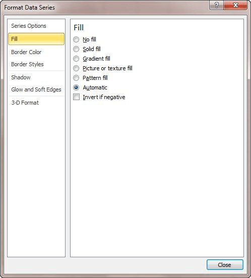
Figure 1. The Format Data Series dialog box.
If you are using Excel 2013, then these steps are for you:
The only element visible at this point is the legend. Keep in mind that the chart is still there, it has just been "hidden" by changing its appearance. This is a long workaround but it gets the job done.
ExcelTips is your source for cost-effective Microsoft Excel training. This tip (8066) applies to Microsoft Excel 2007, 2010, and 2013. You can find a version of this tip for the older menu interface of Excel here: Putting a Chart Legend On Its Own Page.

Dive Deep into Macros! Make Excel do things you thought were impossible, discover techniques you won't find anywhere else, and create powerful automated reports. Bill Jelen and Tracy Syrstad help you instantly visualize information to make it actionable. You�ll find step-by-step instructions, real-world case studies, and 50 workbooks packed with examples and solutions. Check out Microsoft Excel 2019 VBA and Macros today!
When charting your data, a legend is always a nice finishing touch. You may want to change the order in which items ...
Discover MoreNeed to move a chart legend to a different place on the chart? It's easy to do using the mouse, as described in this tip.
Discover MoreWhen you create a chart, Excel often includes a legend with the chart. You can format several attributes of the legend's ...
Discover MoreFREE SERVICE: Get tips like this every week in ExcelTips, a free productivity newsletter. Enter your address and click "Subscribe."
2021-10-07 10:50:09
Ronmio
I should have also mentioned that you can use the Windows Snipping Tool to capture and save the legend for pasting anywhere.
(see Figure 1 below)
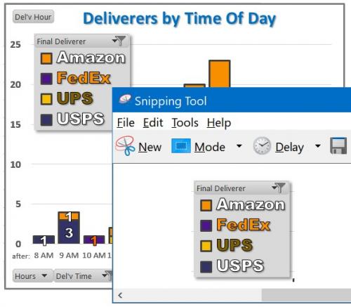
Figure 1.
2021-10-06 10:08:50
d
I don't know about the other people, for me I wanted to copy the legend with the icons on them. The screenshot works better but I have to work with a white background of it. However, the last method is not really useful since when you put every bar in a no-filled mode then you automatically get a nothing legend, with only words. I wanted to put only one legend for different graphs but I want a better place for it, not only inside one single chart.
2020-07-20 11:48:26
Ronmio
There is a much easier way that can be done entirely in Excel in two steps.
Select the chart and use the Copy dropdown on the Home menu to select "Copy as Picture ..." and click on OK to select the defaults. Then paste the picture of the chart where you want it and select Crop on the Format tab* of the Picture Tools to trim away all but the legend. Done.
*That's where Crop is in Excel 2013. In Excel 2019 or Excel 365, the Crop tool will be found under the Picture Format menu.
2015-11-15 19:11:45
Darren E
Rick K, linked picture would be OK as long as it is not a calculation-intensive workbook. Linked pictures can bring large workbooks to a grinding halt.
For this application I would just copy the chart, and in the copy:
1. Select plot area
2. Shrink it by dragging the bottom left sizing handle all the way to the top right.
3. Make the legend opaque and put it over the top of the plot area.
2015-11-12 09:02:24
Rick K
Another way is to use the camera tool and paste the linked picture to a separate sheet.
Got a version of Excel that uses the ribbon interface (Excel 2007 or later)? This site is for you! If you use an earlier version of Excel, visit our ExcelTips site focusing on the menu interface.
FREE SERVICE: Get tips like this every week in ExcelTips, a free productivity newsletter. Enter your address and click "Subscribe."
Copyright © 2026 Sharon Parq Associates, Inc.
 Please Note:
This article is written for users of the following Microsoft Excel versions: 2007, 2010, and 2013. If you are using an earlier version (Excel 2003 or earlier), this tip may not work for you. For a version of this tip written specifically for earlier versions of Excel, click here:
Please Note:
This article is written for users of the following Microsoft Excel versions: 2007, 2010, and 2013. If you are using an earlier version (Excel 2003 or earlier), this tip may not work for you. For a version of this tip written specifically for earlier versions of Excel, click here:
Comments