Hiding and Protecting Columns

Roger has a worksheet that he needs to distribute to different people so they can add and change some information. He wants to hide some of the columns in the worksheet, however, so that they cannot be viewed by users. He knows how to protect the worksheet and how to hide data in cells but noticed that info is still visible in the formula bar.

Since you already know how to protect a worksheet, you are already on your way to accomplishing your task. These are the steps you should follow:

1. Select the column you want to protect.
2. Press Ctrl+Shift+F. Excel displays the Format Cells dialog box.
3. Make sure the Protection tab is displayed. (See Figure 1.)



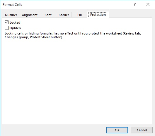
Figure 1. The Protection tab of the Format Cells dialog box.

4. Make sure both the Locked and Hidden check boxes are selected. (It is the Hidden check box that controls whether the cell contents are visible in the formula bar or not.)
5. Click OK to dismiss the dialog box.
6. With the column still selected, display the Home tab of the ribbon.
7. Starting in the Cells group, click Format | Hide & Unhide | Hide Columns. Excel hides the column.
8. Again, starting in the Cells group, click Format | Protect Sheet. Excel displays the Protect Sheet dialog box. (See Figure 2.)



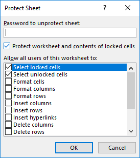
Figure 2. The Protect Sheet dialog box.

9. Enter a password to be used in protecting the worksheet.
10. Using the check boxes, select what type of protection you want applied to the worksheet. At a minimum you should choose Select Locked Cells and Select Unlocked Cells. (These two options are selected by default in a worksheet.)
11. Click OK to dismiss the dialog box. You are prompted to reenter your password (the one from step 9), which you should do.

At this point someone cannot view what is in the hidden column, even if they use F5 to jump to one of the cells in the column; it still won't appear in the formula bar. There is one caveat to all this: If you have some cells in the worksheet (or workbook) that are unlocked, so that the contents of the cell can be changed, it is still possible to see what is in individual cells of the column. How? Two methods, really:

• In the unlocked cell, enter a formula that references a locked and hidden cell. For instance, if column E is locked and hidden, entering the formula =E3 will display, in the unlocked cell, the value in cell E3.
• Copy the contents of the locked and hidden cell and paste it in the unlocked cell. Use F5 to jump to the locked and hidden cell, then press Ctrl+C, move to the unlocked cell, and press Ctrl+V. The contents of the locked and hidden cell are pasted in the unlocked cell.

The bottom line is that it is virtually impossible to 100% protect the contents of the column so that they cannot be viewed. Using the protection features of Excel makes it more difficult, but a determined user may be able to still view the contents in the described manner.

ExcelTips is your source for cost-effective Microsoft Excel training. This tip (8069) applies to Microsoft Excel 2007, 2010, 2013, 2016, 2019, and Excel in Microsoft 365. You can find a version of this tip for the older menu interface of Excel here: Hiding and Protecting Columns.