Please Note: This article is written for users of the following Microsoft Excel versions: 2007, 2010, 2013, 2016, 2019, 2021, and Excel in Microsoft 365. If you are using an earlier version (Excel 2003 or earlier), this tip may not work for you. For a version of this tip written specifically for earlier versions of Excel, click here: Multiple Print Areas on a Single Printed Page.
Written by Allen Wyatt (last updated July 27, 2024)
This tip applies to Excel 2007, 2010, 2013, 2016, 2019, 2021, and Excel in Microsoft 365
Ingrid set up her worksheet just the way she wanted, and then defined two non-contiguous areas on the worksheet as her print area. She first selected A1:C5, then held down the Ctrl key as she selected E3:G5. This selection was then defined as the print area. When Ingrid printed the worksheet, each of the selected ranges (A1:C5 and E3:G5) printed, but they printed on separate sheets of paper. Ingrid was hoping to get them on a single sheet of paper.
This happens because Excel automatically prints separate ranges on separate sheets of paper; there is no way to configure Excel to do this printing differently. There are a couple of things you can try as workarounds, however.
First, you could print multiple pages per sheet of paper. Follow these steps:
The result, for most printers, is that Excel combines two printed pages on a single sheet of paper. It does this by reducing the size of each of the two pages and printing them in landscape mode on the page. If you cannot find a control that allows you to specify multiple pages per sheet (step 5), it may be that your printer driver doesn't offer this capability. In that case, you won't be able to use this workaround and will have to try the next one.
The next solution involves simply creating a "print" worksheet. This sheet can contain references to the original data ranges, combining them on a single worksheet. You can then print the consolidation worksheet, as it will contain only the information you want sent to the printer.
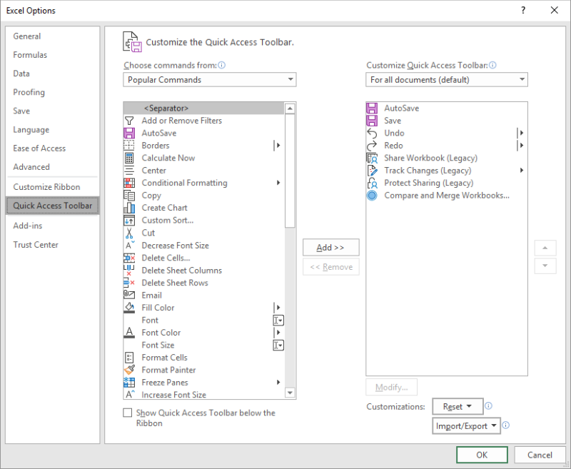
A third option involves using the Camera tool. This tool allows you to capture dynamic "pictures" of different areas of your worksheet. The Camera tool is not available, by default, on any of Excel's ribbons. Instead, you need to add it to the Quick Access Toolbar:

Figure 1. The Quick Access Toolbar option in the Excel Options dialog box.
You are now ready to use the Camera tool. Follow these steps:
Now you can manipulate the two pictures the same as you would any other graphic—stretch, resize, crop, or move them; whatever. The picture is not really a picture, however, even though it behaves as one. Instead, it is dynamic, meaning that if the contents of the original ranges are changed, then what is shown in the picture changes, as well. You can also print the worksheet containing the camera pictures, and they will appear on a single page.
ExcelTips is your source for cost-effective Microsoft Excel training. This tip (8189) applies to Microsoft Excel 2007, 2010, 2013, 2016, 2019, 2021, and Excel in Microsoft 365. You can find a version of this tip for the older menu interface of Excel here: Multiple Print Areas on a Single Printed Page.

Solve Real Business Problems Master business modeling and analysis techniques with Excel and transform data into bottom-line results. This hands-on, scenario-focused guide shows you how to use the latest Excel tools to integrate data from multiple tables. Check out Microsoft Excel Data Analysis and Business Modeling today!
Many people, when they print a worksheet, print the entire thing. You don't have to, however. You can specify that Excel ...
Discover MoreExcel allows you to specify a print range that defines what should be printed from a given worksheet. This tip shows how ...
Discover MorePrint areas are a great way to define what, exactly, you want to print from a worksheet. When you copy worksheets, the ...
Discover MoreFREE SERVICE: Get tips like this every week in ExcelTips, a free productivity newsletter. Enter your address and click "Subscribe."
2026-01-22 16:22:45
Sandeep
Very useful
2024-07-27 10:02:38
J. Woolley
For an equivalent of the Camera tool, copy (Ctrl+C) a region of the active sheet, then select another cell on any sheet and pick Home > Paste > Linked Picture (Alt+H+V+I).
My Excel Toolbox includes the following two macros to create an image of a range of cells. In addition to cell values, the images will include visible portions of shapes or charts from the copied range.
1. SelectionImage copies the selected range as a static image on the clipboard and optionally saves it in a file.
2. DynamicImage copies the selected range and pastes it as a dynamic image in any sheet of any workbook. All changes visible in the source range will be reproduced in the dynamic image (assuming the source is open in Excel). The result is a simple dashboard.
See https://sites.google.com/view/MyExcelToolbox/
Got a version of Excel that uses the ribbon interface (Excel 2007 or later)? This site is for you! If you use an earlier version of Excel, visit our ExcelTips site focusing on the menu interface.
FREE SERVICE: Get tips like this every week in ExcelTips, a free productivity newsletter. Enter your address and click "Subscribe."
Copyright © 2026 Sharon Parq Associates, Inc.
Comments