Segregating Numbers According to Their Sign

Are you working with a large set of data consisting of mixed values, some negative and some positive, that you want to separate into columns based on their sign? There are a few ways this can be approached. One method is simply to use a formula in the columns to the right of the mixed column. For instance, if the mixed column is in column A, then you could place the following formula in the cells of column B:

=IF(A2>0,A2,0)

This results in column B only containing values that are greater than zero. In column C you could then use this formula:

=IF(A2<0,A2,0)

This column would only contain values less than zero. The result is two new columns (B and C) that are the same length as the original column. Column B is essentially the same as column A, except that negative values are replaced by zero, while column C replaces positive values with zero.

If you want to end up with columns that only contain negative or positive values (no zeroes), then you can use the filtering capabilities of Excel. Assuming you are using Excel 2021, 2024, or Excel 365 and that the mixed values are in column A, you can use the following formulas in cells B2 and C2, respectively:

=FILTER(A2:A999,A2:A199>0)
=FILTER(A2:A999,A2:A199<0)

You should replace the range in the formulas (A2:A999) with the actual range of values in column A. If you are using an older version of Excel, then you can use the advanced filtering capabilities of the program. Follow these steps:

1. If you have a column heading in cell A1, copy it to cell E1.
2. In cell E2, place the formula >0.
3. Select any cell in the mixed values of column A.
4. Display the Data tab of the ribbon.
5. Click Advanced in the Sort & Filter group. Excel displays the Advanced Filter dialog box. The List Range should already be filled in, representing the range of mixed values in Column A. (See Figure 1.)



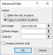
Figure 1. The Advanced Filter dialog box.

6. Make sure the Copy to Another Location radio button is selected.
7. Select the Criteria Range box and then use the mouse to select cells E1:E2. This tells Excel that you only want cells in the original range that are greater than zero.
8. Select the Copy To box and click once in cell B1.
9. Click on OK. Column B now contains cells that are greater than zero.
10. In cell E2, place the formula <0.
11. Again, display the Data tab of the ribbon.
12. Click again on the Advanced tool in the Sort & Filter group. Excel displays the Advanced Filter dialog box. The settings in the dialog box should be the same as the last time you used them.
13. Select everything in the Copy To box, and then click once in cell C1.
14. Click on OK. Column C now contains cells that are less than zero.

You now have the desired two columns of positive and negative values. You can also delete the cells at E1:E2 if you desire.

ExcelTips is your source for cost-effective Microsoft Excel training. This tip (9601) applies to Microsoft Excel 2007, 2010, 2013, 2016, 2019, 2021, 2024, and Excel in Microsoft 365. You can find a version of this tip for the older menu interface of Excel here: Segregating Numbers According to Their Sign.