Finding Odd Values Greater Than 50

Amol has 1,000 values in an Excel worksheet, occupying 100 rows of 10 columns each. Each value in this range is an integer value between 0 and 99. Amol needs a way to count and display all the values which are odd and greater than 50.

There are a few ways you can go about counting and displaying, but it is important to understand that these are different tasks. Perhaps the best way to display those values that fit the criteria is to use conditional formatting. You can add a conditional formatting rule to each cell that will make bold or otherwise highlight the desired values. Follow these steps:

1. Select the cells that contain your data.
2. Display the Home tab of the ribbon.
3. Click the Conditional Formatting tool in the Styles group. Excel displays a palette of options related to conditional formatting.
4. Click New Rule. Excel displays the New Formatting Rule dialog box. (See Figure 1.)



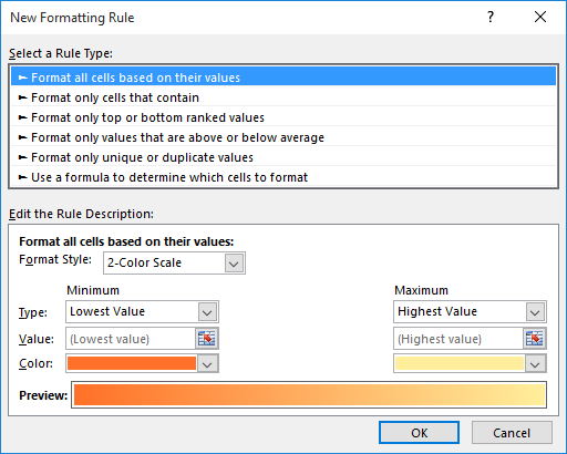
Figure 1. The New Formatting Rule dialog box.

5. In the Select a Rule Type area at the top of the dialog box, choose Use a Formula To Determine Which Cells to Format.
6. In the formula box enter the formula =AND(MOD(A1,2),A1>50).
7. Click the Format button. Excel displays the Format Cells dialog box. (See Figure 2.)



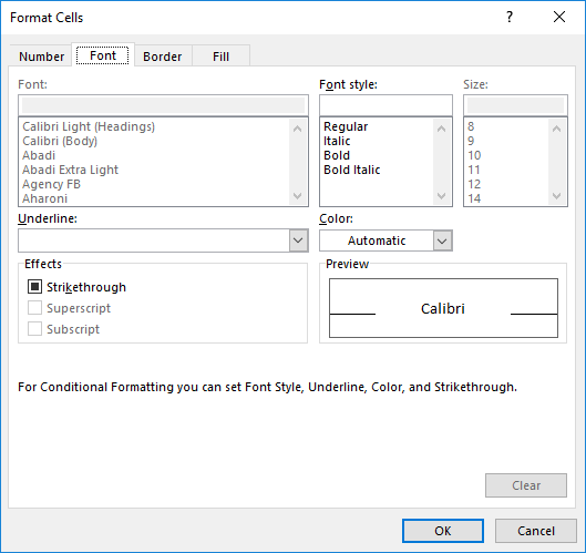
Figure 2. The Format Cells dialog box.

8. Use the controls in the dialog box to modify the formatting, as desired.
9. Click OK to close the Format Cells dialog box.
10. Click OK to close the New Formatting Rule dialog box. The formatting is applied to the range of cells you selected in step 1.

If you prefer, you could also use the following formula in step 6:

=AND(ISODD(A1),A1>50)

To get the count of cells that fit the criteria, you could use an array formula:

=SUM(MOD(MyCells,2)*(MyCells>50)

This formula assumes that the range of cells you want to analyze are named MyCells. Don't forget to enter the cell using Ctrl+Shift+Enter. If you don't want to use an array formula, you could use the following:

=SUMPRODUCT((MOD(MyCells,2)*(MyCells>50))

You could also use a macro to derive both the cells and the count. The following is a simple version of such a macro; it places the values of the cells matching the criteria into column M and then shows a count of how many cells there were:

Sub SpecialCount()
    Dim c As Range
    Dim i As Integer

    i = 0
    For Each c In Range("A2:J101")
        If c.Value > 50 And c.Value Mod 2 Then
            i = i + 1
            Range("L" & i).Value = c.Value
        End If
    Next c

    MsgBox i & " values are odd and greater than 50", vbOKOnly
End Sub

ExcelTips is your source for cost-effective Microsoft Excel training. This tip (12597) applies to Microsoft Excel 2007, 2010, 2013, 2016, 2019, and Excel in Microsoft 365.