Terry has a workbook that has numerous named ranges defined. He wonders if there is a way to determine which named ranges are actually used in formulas so that he can delete the names that aren't used.
There are a few different ways this can be accomplished. One easy way is to fire up the Name Manager (press Ctrl+F3) and jot down the names of all the range names you want to check. Close the Name Manager and then follow these steps:
At this point, Excel will display all the cells in which it found the range name you specified in step 2. If nothing is displayed, then the name isn't used in any formulas. You can then repeat the steps for each of the other range names you want to check.
You can make the process more automatic by wrapping the finding process within a macro. The following is an example:
Sub CleanseNames()
    Dim ns As Names
    Dim n As Name

    Set ns = ThisWorkbook.Names
    MsgBox "There are " & ns.Count & " names in the workbook", vbInformation
    For Each n In ns
        On Error GoTo err
        fnd = False
        fnd = Cells.Find(What:=n.Name, LookIn:=xlFormulas, _
          LookAt:=xlPart).Activate
err:
        If fnd = False Then n.Delete
    Next n
End Sub
The macro steps through each range name in the workbook and then looks for that name in any cell. If it is not found, then the name is deleted.
Of course, it may not be in your best interest to automatically delete names. After all, they can be in more places than just formulas. It might be better to simply list those names that aren't apparently in use. Here's an example of a macro that will accomplish the task:
Sub ListUnusedNames()
    Dim w As Worksheet
    Dim n As Name
    Dim sUnusedNames As String
    Dim arrUsedNames() As String
    Dim K As Integer

    On Error Resume Next
    K = -1
    For Each n In Names   ' First Loop
        For Each w In ActiveWorkbook.Worksheets
            If Not w.Cells.Find(What:=n.Name, _
                After:=ActiveCell, LookIn:=xlFormulas, _
                LookAt:=xlPart, SearchOrder:=xlByRows, _
                SearchDirection:=xlNext, MatchCase:=False, _
                SearchFormat:=False) Is Nothing Then

                K = K + 1
                ReDim Preserve arrUsedNames(K)
                arrUsedNames(K) = n.Name
                ' Jump out early; found an occurrence
                GoTo LabNextName
            End If
        Next w
LabNextName:
    Next n

    sUnusedNames = ""
    For Each n In Names   ' Second Loop
        If Not IsPartOfArray(n.Name, arrUsedNames) Then
            sUnusedNames = sUnusedNames & n.Name & vbCr
        End If
    Next n

    If Len(sUnusedNames) = 0 Then
        MsgBox "There are no names in the active workbook that are unused."
    Else
        MsgBox "Unused Names:" & vbCr & vbCr & sUnusedNames
    End If
End Sub
Function IsPartOfArray(stringToBeFound As String, arr As Variant) As Boolean
    'Returns TRUE If argument 'stringToBeFound' is part of array 'arr'.

    IsPartOfArray = Not IsError(Application.Match(stringToBeFound, arr, 0))
End Function
If you prefer to use a third-party solution to managing the names in your workbook—including figuring out which names are unused—a great choice is the Name Manager add-in, written by Jan Karel Pieterse. You can find more information on this free add-in here:
https://jkp-ads.com/excel-name-manager.asp
ExcelTips is your source for cost-effective Microsoft Excel training. This tip (10338) applies to Microsoft Excel 2007, 2010, 2013, 2016, 2019, 2021, and Excel in Microsoft 365.

Professional Development Guidance! Four world-class developers offer start-to-finish guidance for building powerful, robust, and secure applications with Excel. The authors show how to consistently make the right design decisions and make the most of Excel's powerful features. Check out Professional Excel Development today!
ISBN numbers are used to denote a unique identifier for a published book. If you remove the dashes included in an ISBN, ...
Discover MoreDo you need to total all the cells that are a particular color, such as yellow? This tip looks at three different ways ...
Discover MoreWant to add up a bunch of scores, without including the lowest one in the bunch? You can make a small change to your ...
Discover MoreFREE SERVICE: Get tips like this every week in ExcelTips, a free productivity newsletter. Enter your address and click "Subscribe."
2023-11-04 09:25:28
Ron S
There is another similar tip with slightly different macros
https://excelribbon.tips.net/T010998_Finding_Unused_Names.html
2023-03-05 11:35:02
J. Woolley
Re. my comment dated 2023-03-03 (2 days ago), I have finally discovered how to reference MyName with Workbook scope as part of a formula on Sheet1. As described before, a qualified reference to Book1.xlsx!MyName was always replaced by the duplicate name with Sheet scope Sheet1!MyName, and an unqualified reference to MyName (like =MyName) always had the value of Sheet1!MyName (2, not 1). Now I have determined that by arbitrarily using an existing sheet name to qualify MyName (like Sheet2!MyName, assuming there is not a duplicate MyName with Sheet2 scope), Excel will convert it to Book1.xlsx!MyName (that is, MyName with Workbook scope).
This demonstrates one of the idiosyncrasies of using a defined name (named range) with Workbook scope. For more, see my comment dated 2023-03-05 here: https://excelribbon.tips.net/T013427
2023-03-03 16:12:39
J. Woolley
As I was testing the NamesInFormulas macro described in my latest comment below, I discovered a problem using Excel 365. The following scenario demonstrates the issue:
1. Open a new workbook and save it as Book1.xlsx.
2. On Sheet1, enter 1 into cell A1 and 2 into cell B1.
3. Select cell A1, then use Formulas > Define Name to name it MyName with Workbook scope.
4. Select cell B1 and give it the duplicate name MyName with Sheet1 scope.
5. Now open Formulas > Name Manager to review results (see Figure 1 below)
6. In cell E1 start to enter this formula: =My (see Figure 2 below)
7. In the popup dialog, pick MyName (Workbook) and press Tab
(see Figure 3 below) -- Before Enter
8. Now press Enter. Even though =Book1.xlsx!MyName was indicated before, the formula becomes =Sheet1!MyName
(see Figure 3 below) -- After Enter
No matter what I tried, I could not reference MyName with Workbook scope as part of a formula on Sheet1. A qualified reference to Book1.xlsx!MyName always became Sheet1!MyName; an unqualified reference to MyName (like =MyName) always had the value of Sheet1!MyName (2, not 1).
I believe this might derive from a similar problem with the Names object in VBA. With most collection objects (like Workbooks or Worksheets), an Item can be identified by its name or its index number; for example,
Worksheets("Sheet1") or Worksheets(1). Notice Item is the default property of most collection objects.
When names are defined using Formulas > Define Name, each new name is placed at the start of the collection (index number 1). For the Book1.xlsx example above:
ActiveWorkbook.Names(1).Name = "Sheet1!MyName"
ActiveWorkbook.Names(2).Name = "MyName"
ActiveWorkbook.Names("MyName").Name = "Sheet1!MyName"
ActiveWorkbook.Names("Sheet1!MyName").Name = "Sheet1!MyName"
ActiveWorkbook.Names("Book1.xlsx!MyName").Name = "Sheet1!MyName"
Therefore, the only reliable way to identify an Item in Names is by its index number; using its name is problematic if there are duplicate names, one with workbook scope and another with sheet scope. This might result from the fact that a Name with workbook scope does not have a fully qualified name like "Book1.xlsx!MyName" but a simple name like "MyName" instead.
Here is a VBA function to return the index number of a Name object given its name (assuming the active workbook's Names collection):
Function Name_Index(Name As String) As Long
Dim n As Long
With ActiveWorkbook
For n = 1 To .Names.Count
If .Names(n).Name = Name Then
Name_Index = n
Exit For
End If
Next n
End With
End Function
This function returns zero if Name does not exist. For the example above:
Name_Index("MyName") = 2
ActiveWorkbook.Names(Name_Index("MyName")).Name = "MyName"
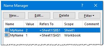
Figure 1.
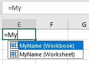
Figure 2.
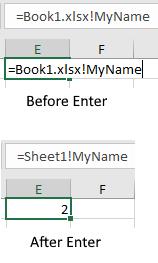
Figure 3.
2023-02-28 17:39:35
J. Woolley
My Excel Toolbox now includes the NamesInFormulas macro, which lists hyperlinks to formula cells referencing each visible defined name (named range) in the active workbook. (Hidden names are ignored.) The cell's formula will be included in a comment attached to its hyperlink. The following details are also provided for each name: Scope, Name, Refers To, Value, and Comment. Results are recorded in the active workbook's 'NamesIn...' worksheet.
The NamesInFormulas macro utilizes the Formula_References function described in my recent comment below.
See https://sites.google.com/view/MyExcelToolbox/
2023-02-27 17:49:54
J. Woolley
The Formula_References function described in my previous comment below has been improved by adding another argument as follows:
Formula_References(Formula, [Remove])
Remove is an optional numeric expression specifying which isolated references should NOT be returned:
0 (default), remove operators and quoted text strings (always);
1, remove numeric constants;
2, remove logical (TRUE/FALSE) constants;
4, remove function names;
8, remove the colon (:) range operator to split cell ranges like $A:$B into $A and $B, which favors named ranges combined like Col.A:Col.B by isolating each defined name.
Add individual values from the above list to remove selected items:
(1+2) to return function names, cell ranges, and defined names
(1+2+4) to return cell ranges and defined names
(1+2+8) to return function names, cell ranges (split), and defined names
(1+2+4+8) to return cell ranges (split) and defined names
Therefore, set Remove=15 to focus on defined names. For the example formula
="Text for today is "&VLOOKUP(TODAY(),Col.A:Col.B,2,FALSE))
Formula_References(Formula, 15) returns the following array A(0 To 1):
{Col.A,Col.B}
See https://sites.google.com/view/MyExcelToolbox/
2023-02-26 10:24:35
J. Woolley
As discussed in this Tip and in previous comments below, there are various ways to determine formula cells that reference a defined name (named range). But invariably it is necessary to examine the formula to verify the particular name of interest is actually referenced therein. This is difficult if the formula contains a quoted text string or the defined name is similar to a function name or the defined name has a duplicate with different scope (workbook or worksheet).
My Excel Toolbox now includes the Formula_References(Formula) function to remove operators and quoted text strings from a cell's formula and return a String array of isolated references including numeric or logical constants, function names, cell ranges, and defined names. Alphabetic case is retained. Function names are distinguished by a trailing left-parenthesis like IF( or VLOOKUP( or TODAY(. Ranges like A1:D4 and apostrophized items like '[My Book.xlsx]Sheet1'!$A$1 or 'My Sheet'!My_Name are returned as is. These isolated references make it easier to determine if a defined name is referenced in a cell's formula.
For example, given the following cell formula that references a two-column range named ODAY (like Sheet1!$A:$B):
="Text for today is "&VLOOKUP(TODAY(),ODAY,2,FALSE))
Formula_References returns the following 5 element base-zero array:
{VLOOKUP(,TODAY(,ODAY,2,FALSE}
If named ranges Col.A and Col.B refer to Sheet1!$A and Sheet1!$B, the previous formula could be written:
="Text for today is "&VLOOKUP(TODAY(),Col.A:Col.B,2,FALSE))
In this case, Formula_References returns the following array A(0 To 4):
{VLOOKUP(,TODAY(,Col.A:Col.B,2,FALSE}
For this example it is necessary to use VBA.Split(A(2),":") to isolate the two named ranges. (Excel's new TEXTSPLIT function or My Excel Toolbox's SplitText function could also be used.)
Here is an abbreviated version of the Formula_References function; useful explanatory comments were removed to fit this space:
Public Function Formula_References(Formula As String) As String()
Const Q As String = """", A As String = "'", X As String = ""
Dim sFormula As String, sS() As String, sT() As String, bA As Boolean
Dim nU As Integer, n As Integer, iU As Integer, i As Integer
ReDim sS(0)
sS(0) = X
Formula_References = sS
sFormula = Formula
If sFormula = X Then Exit Function
sS = Split(sFormula, Q)
If sS(0) <> sFormula Then
nU = UBound(sS)
ReDim sT(0 To (nU \ 2))
For n = 0 To nU Step 2
sT(n \ 2) = sS(n)
Next n
sFormula = Application.Trim(Join(sT))
End If
If sFormula = X Then Exit Function
sS = Split(sFormula, A)
bA = (sS(0) <> sFormula)
If bA Then
nU = UBound(sS)
ReDim sT(0 To (nU \ 2))
For n = 1 To nU Step 2
sT(n \ 2) = sS(n)
sS(n) = ""
Next n
sFormula = Join(sS, vbCr)
End If
If sFormula = X Then Exit Function
sS = Split("+ - * / % ^ = > < >= <= <> & , ) " & vbLf)
nU = UBound(sS)
For n = 0 To nU
sFormula = Replace(sFormula, sS(n), " ")
Next n
sFormula = Replace(sFormula, "(", "( ")
sFormula = Application.Trim(sFormula)
If sFormula = X Then Exit Function
sS = Split(sFormula)
nU = UBound(sS)
For n = 0 To nU
If Left(sS(n), 1) = "(" Then sS(n) = Mid(sS(n), 2)
Next n
sS = Split(Application.Trim(Join(sS)))
If bA Then
nU = UBound(sS)
iU = UBound(sT)
For n = 0 To nU
For i = 0 To iU
sS(n) = Replace(sS(n), (vbCr & vbCr), (A & sT(i) & A), 1, 1)
Next i
Next n
End If
Formula_References = sS
End Function
See https://sites.google.com/view/MyExcelToolbox/
2023-02-12 23:59:56
@J. Woolley:
Your macros run fine on my test workbook, both original and with corrections you posted.
I did not fully grasp your algorithm logic, but they (macros) list the number of cells referencing each defined name only if the name is part of the formula not just part of the text. So you solved this Catch-22-like problem. Very clever use of error count.
Good job.
Also, I must have applied your earlier tip regarding "If n.Visible then..." incorrectly. I tried it in different macro and found that the solver range names are actually hidden, hence they do not show in the list your macro generates. Good job again.
I will keep your macro in my toolbox (with credit to you and note 'inspired by Doug Glancy').
I bet it will come handy one day.
2023-02-12 16:19:32
J. Woolley
Re. the NamesInCells macro in my previous comment below:
The following statements
If IsError(Evaluate(sRefersTo)) _
And Right(sRefersTo, 5) <> "#REF!" Then
vCells = "Indeterminate"
Else
.RefersTo = "#REF!"
vCells = Formula_Errors(WB) - nBase
.RefersTo = sRefersTo
vCells = vCells + Prior_Errors(WB, .Name)
End If
should be replaced by
If Left(sScope, 1) = "'" Then _
sScope = Mid(sScope, 2, (Len(sScope) - 2))
.RefersTo = "#REF!"
vCells = Formula_Errors(WB) - nBase
.RefersTo = sRefersTo
vCells = vCells + Prior_Errors(WB, .Name)
because sScope does not need surrounding apostrophes and the Indeterminate condition is handled by the Prior_Errors function. Also, that function should be replaced by the following:
Private Function Prior_Errors(WB As Workbook, Name As String) As Long
Dim WS As Worksheet, R As Range, rCell As Range, nCount As Long
Dim sWS As String, sN As String, sF As String, n As Integer
n = InStrRev(Name, "!")
If n > 1 Then
sN = Mid(Name, (n + 1))
sWS = Left(Name, (n - 1))
If Left(sWS, 1) = "'" Then sWS = Mid(sWS, 2, (Len(sWS) - 2))
End If
For Each WS In WB.Worksheets
On Error Resume Next
Set R = WS.Cells.SpecialCells(xlCellTypeFormulas, xlErrors)
If Err = 0 Then
For Each rCell In R
sF = rCell.Formula
If WS.Name = sWS Then
If InStr(1, sF, sN, vbBinaryCompare) > 0 Then
nCount = nCount + 1
End If
ElseIf InStr(1, sF, Name, vbBinaryCompare) > 0 Then
nCount = nCount + 1
End If
Next rCell
End If
On Error GoTo 0
Next WS
Prior_Errors = nCount
End Function
I should mention that duplicate Names with separate scope might be counted extraneously if any of them are in a formula that had an error before the macro was initiated
2023-02-11 19:54:07
Tomek
@J. Woolley 2023-02-11 15:51:07
Re: 1. You are right. Whatever you do, there is a gotcha in this puzzle,
Re: 2. I tried it, it did not work. I do not know how these Solver names are added to the workbook, but they only show up in the workbook after the solver was invoked, even if it was not run, but not before.
The names show in the MsgBox from the macro, but I couldn't find them anywhere, they do not show up in the Name Manager, nor in the name Box.
You cannot type them into the GoTo dialog box. I wonder if they are names of other objects, not ranges.
Anyway, this is quite academic, I only posted it as a warning that the macro may list more names than expected.
2023-02-11 15:58:01
J. Woolley
For more on this subject, see https://excelribbon.tips.net/T003153_Identifying_Unused_Named_Ranges.html
2023-02-11 15:51:07
J. Woolley
@Tomek
1. Suppose you define MyName that refers to cell $A$1. If you trace dependents of $A$1, you still must use Find or InStr to determine whether the dependent is a formula that references MyName (like =MyName) or simply references $A$1 (like =$A$1).
2. In your Figure 1, are the solver_... names hidden? If so, you could modify the Tip's macro by adding
If n.Visible Then
...
End If
2023-02-11 15:07:37
J. Woolley
The following NamesInCells macro reports the number of formula cells referencing each defined name (named range) in the active workbook. Results are in columns A:D (Scope, Name, RefersTo, Cells) starting at row 1 of the workbook's NamesInCells worksheet. If that worksheet does not exist, it will be added after the last sheet.
For each Name that is Visible (not hidden), the macro uses Private Function Formula_Errors to determine how many formula cells have errors before and after the Name's RefersTo property is made invalid. The before and after difference is the number of cells referencing that Name in a formula. However, if a Name is used in a cell formula that produced an error before, the after result will be the same for that cell. This issue is resolved by Private Function Prior_Errors which determines if the Name appears in an error cell's formula before the Name was made invalid. The InStr method used by Prior_Errors is similar to the Tip's Find method; therefore, it is imperfect as described in my earlier comment, but only for formulas that had errors before initiating the macro (hopefully few).
Notice that some Names are reported as Indeterminate before changing their RefersTo property; for example, this applies to a valid Name that RefersTo an external workbook that is not currently open.
This macro was inspired by Doug Glancy, https://stackoverflow.com/a/26691025/10172433.
Public Sub NamesInCells()
Const myName As String = "NamesInCells"
Dim WB As Workbook, oName As Name, A() As Variant, vCells As Variant
Dim sScope As String, sName As String, sRefersTo As String
Dim nRows As Long, nR As Long, nBase As Long, n As Integer
Set WB = ActiveWorkbook
nRows = WB.Names.Count
If nRows = 0 Then
MsgBox "There are no defined names in the active workbook", _
vbInformation, myName
Exit Sub
End If
nRows = nRows + 1
ReDim A(1 To 4, 1 To nRows)
nR = 1
A(1, 1) = "Scope"
A(2, 1) = "Name"
A(3, 1) = "RefersTo"
A(4, 1) = "Cells"
nBase = Formula_Errors(WB)
For Each oName In WB.Names
With oName
If .Visible Then 'skip hidden names
n = InStrRev(.Name, "!")
If n = 0 Then
sScope = "Workbook"
sName = .Name
ElseIf n > 1 Then
sScope = Left(.Name, (n - 1))
sName = Mid(.Name, (n + 1))
End If
sRefersTo = .RefersTo
If IsError(Evaluate(sRefersTo)) _
And Right(sRefersTo, 5) <> "#REF!" Then
vCells = "Indeterminate"
Else
.RefersTo = "#REF!"
vCells = Formula_Errors(WB) - nBase
.RefersTo = sRefersTo
vCells = vCells + Prior_Errors(WB, .Name)
End If
nR = nR + 1
A(1, nR) = sScope
A(2, nR) = sName
A(3, nR) = "'" & sRefersTo
A(4, nR) = vCells
End If
End With
Next oName
If nR < 2 Then
MsgBox "There are no visible defined names in the active workbook", _
vbInformation, myName
Exit Sub
ElseIf nR < nRows Then
ReDim Preserve A(1 To 4, 1 To nR)
End If
On Error Resume Next
With WB
.Worksheets(myName).Activate
If Err = 0 Then
Range("A:D").Clear
Else
.Worksheets.Add After:=.Sheets(.Sheets.Count)
ActiveSheet.Name = myName
End If
End With
On Error GoTo 0
Range("A1").Select
Selection.Resize(nR, 4).Value = Application.Transpose(A)
End Sub
Private Function Formula_Errors(WB As Workbook) As Long
Dim WS As Worksheet, R As Range, nCount As Long
For Each WS In WB.Worksheets
On Error Resume Next
Set R = WS.Cells.SpecialCells(xlCellTypeFormulas, xlErrors)
If Err = 0 Then nCount = nCount + R.Count
On Error GoTo 0
Next WS
Formula_Errors = nCount
End Function
Private Function Prior_Errors(WB As Workbook, Name As String) As Long
Dim WS As Worksheet, R As Range, rCell As Range, nCount As Long
For Each WS In WB.Worksheets
On Error Resume Next
Set R = WS.Cells.SpecialCells(xlCellTypeFormulas, xlErrors)
If Err = 0 Then
For Each rCell In R
If InStr(1, rCell.Formula, Name, vbBinaryCompare) > 0 Then
nCount = nCount + 1
End If
Next rCell
End If
On Error GoTo 0
Next WS
Prior_Errors = nCount
End Function
2023-02-11 12:56:34
I stumbled upon another problem in the second macro from the tip: it shows range names that are part of Excel Add-ins, in my case part of Solver. (see Figure 1 below)
Not that the information given is incorrect, but it is confusing by adding irrelevant name ranges.
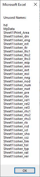
Figure 1.
2023-02-11 12:46:44
J. Woolley:
It is definitely a problem, because ranges that are not used a part of the formula will be identified as used. I wrote a similar macro and it had the same problem, but at least this approach will not lead to deleting the names that are actually used in the formulas.
I tried to modify my macro to eliminate the text finds, but failed; the logic became very complex and I gave up.
My thought was to activate each named range and look for dependents, to decide if the name is used, but run out of time before sending my suggestion to Allen.
I stumbled upon another problem with Allen's second macro. See my next comment
2023-02-11 10:41:38
J. Woolley
The Tip's suggestions ignore the fact that the Name of a named range might also appear in a cell's formula as part of a text string or the name of a function. For example, suppose you give cell Sheet1!$D$1 the name Today (or TODAY) and give cell Sheet1!$D$2 the name Text (or TEXT). Now suppose cells $D$1 and $D$2 have the following formulas:
="Today is "&TEXT(TODAY(),"mm/dd/yyyy")
="Text for today is "&VLOOKUP(TODAY(),$A:$B,2,FALSE)
The Tip's methods would declare that both formulas contain both named ranges Today (or TODAY, or even ToDaY) and Text (or TEXT, or even TeXt), but they don't. Here are some more named ranges that would mistakenly be identified in these formulas: Oday, Ext, Look, ALS, etc.
The Tip's macros could be improved by changing the Find statements to include MatchCase:=True, but that still would not guarantee correct results for the previous example nor for these potential named ranges: oday, ODAY, ext, EXT, etc.
Got a version of Excel that uses the ribbon interface (Excel 2007 or later)? This site is for you! If you use an earlier version of Excel, visit our ExcelTips site focusing on the menu interface.
FREE SERVICE: Get tips like this every week in ExcelTips, a free productivity newsletter. Enter your address and click "Subscribe."
Copyright © 2026 Sharon Parq Associates, Inc.
Comments