Please Note: This article is written for users of the following Microsoft Excel versions: 2007 and 2010. If you are using an earlier version (Excel 2003 or earlier), this tip may not work for you. For a version of this tip written specifically for earlier versions of Excel, click here: Checking for Duplicate Rows Based on a Range of Columns.
Jennifer has a lot of data in a worksheet, and she considers some of the rows to be duplicates. She determines whether a row is a duplicate based upon whether a range of columns in one row is identical to the same range of columns in the previous row. For instance, if all of the values in F7:AB7 are identical to the values in F6:AB6, the Jennifer would consider row 7 to be a duplicate of row 6. She wonders if there is a way that she can easily check for such duplicate rows and highlight the duplicates in some manner.
One approach to this problem is to utilize the conditional formatting capabilities of Excel. If your data is in rows A1:AZ100, then select the range You could then use the following as a formulaic test within your conditional format:
=IF(AND($F2:$AB2=$F1:$AB1),1,0)=1
If your conditional format applies a color to the cells, then you'll see the color appear anytime the values in columns F through AB are equal to the values in the same columns of the row directly above the one that is colored.
If Jennifer's data consists only of cells in the columns F:AB, then she can use the filtering capabilities of Excel to mark the duplicate rows. Here are the general steps:
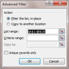
Figure 1. The Advanced Filter dialog box.
At this point, only the duplicate records are highlighted with the color you used in step 2. These records can be safely deleted, leaving only the unique records.
Perhaps an even easier approach is to allow Excel to determine the duplicates and remove the rows. Follow these steps:
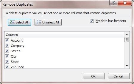
Figure 2. The Remove Duplicates dialog box.
The powerful feature of using the Remove Duplicates tool is that the order of the records in the table don't really matter. In other words, the tool doesn't just compare the specified columns in one row to the row above it—it compares the specified columns in one row to all the other rows and it keeps only those that are unique.
ExcelTips is your source for cost-effective Microsoft Excel training. This tip (10608) applies to Microsoft Excel 2007 and 2010. You can find a version of this tip for the older menu interface of Excel here: Checking for Duplicate Rows Based on a Range of Columns.

Best-Selling VBA Tutorial for Beginners Take your Excel knowledge to the next level. With a little background in VBA programming, you can go well beyond basic spreadsheets and functions. Use macros to reduce errors, save time, and integrate with other Microsoft applications. Fully updated for the latest version of Office 365. Check out Microsoft 365 Excel VBA Programming For Dummies today!
If you want to limit what is returned by a formula to something between lower and upper boundaries, the solution is to ...
Discover MoreIf you have a mixture of text, numbers, and blank cells in a column, you may want to determine the address of the first ...
Discover MoreThe precision of numeric values you display in a worksheet can be less than what is actually maintained by Excel. This ...
Discover MoreFREE SERVICE: Get tips like this every week in ExcelTips, a free productivity newsletter. Enter your address and click "Subscribe."
2020-04-04 19:48:19
Sara
Hello
I am working on a document that has numbers in multiple rows and columns. Within each row i have numbers listed, 1-30 and each numbers is associated to a column. I figured out how to use the duplicate value option but instead of treating each row separate it lumps them together. I need each row to be treated separate. For example, lets say row D4: AU4 has numbers 1-30 in it but D5:AU5 also has those same numbers in it. I need each row to show duplicates within that row. How do I get this feature to work with out manually going to each row and applying it there?
Thanks
sara
2018-09-29 17:05:30
Faisal Theyab
You can highlight or delete duplicated or identical rows easily using Dose for Excel Add-In which provides more than +100 Features, check their website in below:
https://www.zbrainsoft.com/excel-delete-rows.html
2015-06-17 09:44:01
Brandon
Hi, I tried this formula and cannot adjust it to do what I need it to do. Is it possible to say IF a value in this column repeats and has the same value in another column then highlight the cell or put true in third column?
=IF(($B2:$B$30000AND$F2:$F$30000),1,0)=1
I have 300,000 records so values in (F) repeat but I am only looking for the ones that repeat on the same account# (B)
2014-12-15 06:34:32
jim
I am trying to write a conditional format for duplicate values. I use 2010 Excel to create a biweekly employee roster. There are times I enter duplicate position assignments and don't catch the error immediately.
I have been trying to write a dynamic rule that as I enter the data if I enter a duplicate it will notify me with a distinct color.
Any help would be appreciated.
2014-04-04 18:21:08
Chuck Trese
@Bryan, ahhh, mia culpa! Yeah, it seems it needs that AND() to keep Excel from trying to re-interpret the equation as text. I did test it before I posted, so now I'm not sure how i got it working - or tricked myself into thinking it was working.
2014-04-04 06:54:22
Bryan
@Chuck: Actually, that's not working for me. It's not comparing each element of the first array to the respective element in the second array; instead, it only highlights the rows when the *first* elements match.
2014-04-03 10:32:13
Neil
We have found that the Remove Duplicates feature keeps the top row of a set of duplicates, so if you have something like a list of chemicals with various daily quantities and you want to remove duplicate chemical listings but keep the largest daily use, sort by use largest to smallest and then Remove Duplicates for chemical name.
2014-04-03 08:58:49
Chuck Trese
Actually, for the conditional format formula, you only need:
=$F2:$AB2=$F1:$AB1
Personally, I would add parentheses, just to make it easier to understand what is going on:
=($F2:$AB2=$F1:$AB1)
2014-04-03 08:35:38
Bryan
AND already returns TRUE/FALSE, so you can simplify your expression to =AND($F2:$AB2=$F1:$AB1). Even if it didn't, IF lets you return TRUE/FALSE, so you could have just said =IF(AND($F2:$AB2=$F1:$AB1),TRUE,FALSE). There's no reason to ever use the IF(something,1,0)=1 construct.
2013-04-02 09:20:26
This might work also:
• highlight the rows (or range) to check,
• click function key F5 (Go To),
• click the Special button at bottom left,
• select Row differences,
• any duplicate rows are highlighted.
Got a version of Excel that uses the ribbon interface (Excel 2007 or later)? This site is for you! If you use an earlier version of Excel, visit our ExcelTips site focusing on the menu interface.
FREE SERVICE: Get tips like this every week in ExcelTips, a free productivity newsletter. Enter your address and click "Subscribe."
Copyright © 2026 Sharon Parq Associates, Inc.
 Please Note:
This article is written for users of the following Microsoft Excel versions: 2007 and 2010. If you are using an earlier version (Excel 2003 or earlier), this tip may not work for you. For a version of this tip written specifically for earlier versions of Excel, click here:
Please Note:
This article is written for users of the following Microsoft Excel versions: 2007 and 2010. If you are using an earlier version (Excel 2003 or earlier), this tip may not work for you. For a version of this tip written specifically for earlier versions of Excel, click here:
Comments