Importing CUSIP Numbers Correctly

Patrick works in the financial sector, and he often has to import files to Excel. Many times these files contain, as one of many fields, what is referred to as a CUSIP number. This value is nine characters long and can contain both letters and digits. When importing, Excel drops any leading zeros, and if there is a letter E near the end of the value, Excel may convert the value to scientific notation. Patrick needs the CUSIP numbers to be imported without modification, so he wonders if there is an elegant (and easy) way to do this.

There are actually three approaches you can use to get the information in that you want. All of the methods assume that you are working with a text file that was output by some other system, other than Excel. The idea behind the approaches is to make sure that Excel, during the import, identifies the field containing the CUSIP numbers as text, instead of trying to convert the field content to numeric values.

Modify the Source

The first method is to modify the source file that you are working with. This could be as easy as talking to whoever controls the software that creates the import file. If you can get them to change how the CUSIP number is generated so that, in the file, the number is preceded by an apostrophe, then importing should be a snap. The apostrophe informs Excel that the field is text, and it will treat it accordingly. Plus, the apostrophe won't show up on the imported data once it is in a worksheet.

You could also load the source file in a text editor and add the apostrophes yourself, but this may be a quite tedious task if there are many records in the file or if you need to work with many files over time.

Modify Your Traditional Import

Again, assuming you are importing a delimited file (either comma delimited to tab delimited), then you can follow these steps to have the file imported correctly:

1. Rename the import file so it has a .TXT filename extension. This step is often overlooked, but it will force Excel to display the Text Import Wizard, which is what you want to have happen.
2. In Excel, display the Open dialog box. (In Excel 2007, click the Office button and then click Open. In Excel 2010, click the File tab of the ribbon and then click Open. In Excel 2013, click the File tab of the ribbon, click Open, then Computer, and finally Browse. In later versions of Excel, click the File tab of the ribbon and click Browse.)
3. Using the Files of Type drop-down list at the bottom of the dialog box, indicate that you want to open Text Files (*.prn; *.txt; *.csv).
4. Locate and select the file you renamed in step 1.
5. Click on Open. Excel starts the Text Import Wizard, displaying the Step 1 of 3 dialog box. (See Figure 1.) (If the Text Import Wizard doesn't start, then you either aren't trying to import a text file or you didn't rename it as indicated in step 1.)



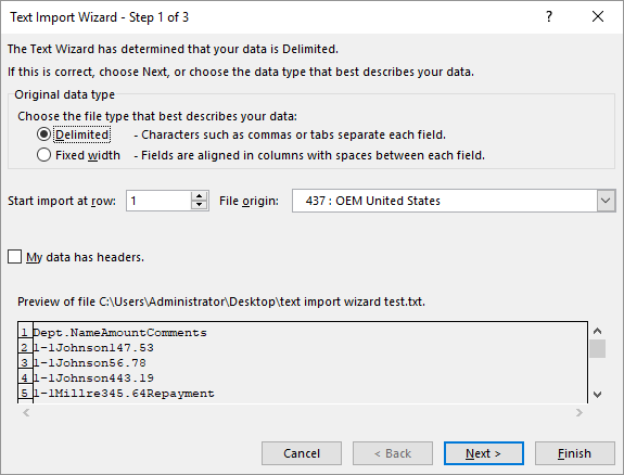
Figure 1. The Text Import Wizard.

6. Make sure the Delimited choice is selected, then click on Next. Excel displays the Step 2 of 3 dialog box.
7. Make sure that either Comma or Tab are selected as a delimiter (depending on your file), then click on Next. Excel displays the Step 3 of 3 dialog box.
8. At the bottom of the dialog box, click on the field that contains your CUSIP numbers. The entire column should now be selected.
9. In the Column Data Format area, make sure the Text radio button is selected.
10. Repeat steps 8 and 9 for any other fields that might confuse Excel. (For instance, if you data has additional CUSIP number fields.)
11. Click on Finish. Your file is imported, and your CUSIP numbers should be intact.

Use Power Query to Import the Data

Assuming you are using at least Excel 2016, you can use Power Query to load your data. Power Query seems to be all the rage these days, and it really does make the importation of data quite easy. Just follow these general steps:

1. Display the Data tab of the ribbon.
2. In the Get & Transform Data group (left side of the ribbon), click From Text/CSV. Excel displays the Import Data dialog box. This looks very much like a standard Open dialog box.
3. Using the controls in the dialog box, locate and select the source file that you want to import.
4. Click Import. Excel "connects" to the data file and, shortly, displays a portion of your data in a large dialog box.
5. Click the Transform button. Excel displays the Power Query Editor dialog box.
6. Check to make sure that the appropriate columns (including the column containing your CUSIP numbers) are being interpreted as text. You can change these, as necessary.
7. Click File | Close & Load To. Excel displays the Import Data dialog box.
8. Make changes in the import settings, as desired. (For most uses, the defaults of Table and New Worksheet should be fine.)
9. Click OK. Excel imports the data from the source file, placing it in a new worksheet.

ExcelTips is your source for cost-effective Microsoft Excel training. This tip (13887) applies to Microsoft Excel 2007, 2010, 2013, 2016, 2019, and Excel in Microsoft 365.