Unique Date Displays

Jon requested help on how to subtract two dates and display the result such that the years were on the left of the decimal and the months on the right. Thus, if you subtracted January 7, 1991 from August 12, 2019, the result would be 28.7.

The easiest way to do this is to simply do your date subtractions as regular, and then use a custom format to display the result. For instance, if the lower date were in cell A2 and the higher date in B2, you could use the following formula in C2:

=B2-A2

You would then follow these steps to format the display of the result in cell C2:

1. Select the cell. (In this case, cell C2.)
2. Display the Home tab of the ribbon.
3. Click the small icon at the lower-right corner of the Number group. Excel displays the Format Cells dialog box.
4. Make sure the Number tab is selected. (See Figure 1.)



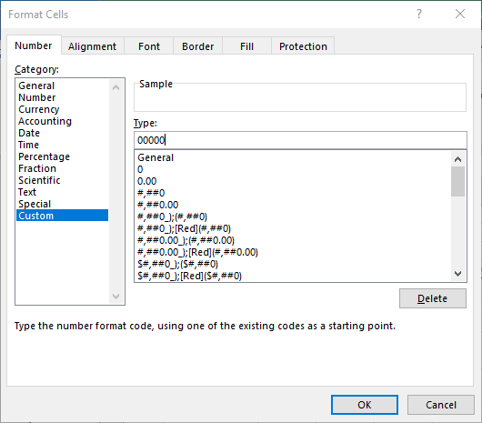
Figure 1. The Number tab of the Format Cells dialog box.

5. In the Category list, at the left side of the dialog box, choose Custom.
6. In the Type box, at the left of the dialog box, enter the following format: yy.m
7. Click on OK.

The result is that C2 shows the number of years to the left of the decimal and the number of months to the right. The problem with this is that it will always vary the number of months from 1 to 12, rather than 0 to 11, as one would expect if you were looking for elapsed months. (Hence, the result of 28.8 in C2.)

To overcome this, you could enter the following formula in cell C2:

=(YEAR(B2)-YEAR(A2))+(MONTH(B2)-MONTH(A2))/100

This formula returns the number of years on the left of the decimal and the number of months on the right. (The result is 28.07 in C2.) There are two potential problems with this approach. First, it won't give the right result if the date in A2 is after the date in B2, particularly if the dates are in different years. (You'll end up with negative years that way.) The second problem is that the months are always expressed using two decimal places, and you may want to not have any leading zeroes.

Both issues can be solved by modifying your formula to use the DATEDIF function, returning the result as text instead of as a numeric value, in this manner:

=IF(A2 < B2, DATEDIF(A2,B2,"y") & "." & DATEDIF(A2,B2,"ym"), DATEDIF(B2,A2,"y") & "." & DATEDIF(B2,A2,"ym"))

There are two variations of the DATEDIF function in this formula, wrapped in an IF function. The reason is because DATEDIF expects the first parameter to be earlier than the second parameter, and the IF function checks to make sure this is the case.

The result in C2 is now 28.7, but it is a text string, not a numeric value. It is necessary to return a text string because a difference of 1 and 10 months would both return as something like 28.1 if the result were numeric.

ExcelTips is your source for cost-effective Microsoft Excel training. This tip (11057) applies to Microsoft Excel 2007, 2010, 2013, 2016, 2019, 2021, and Excel in Microsoft 365. You can find a version of this tip for the older menu interface of Excel here: Unique Date Displays.