Written by Allen Wyatt (last updated February 12, 2022)
This tip applies to Excel 2007, 2010, 2013, 2016, 2019, 2021, and Excel in Microsoft 365
Excel includes a Remove Duplicates tool which can be useful. Ulises, however, would like to simply identify the duplicates rather than remove them. He wonders if there is an "Identify Duplicates" tool of some type.
One way that many people use (including myself) is to rely on a helper column. Let's say that you want to check for duplicates based on the contents of column C, and that row 1 contains headers for each of the column. This means that your data begins in cell C2.
First, sort your data by column C. Then, in a different, unused column (let's say that is column F), insert the following into cell F3, which corresponds with the second row of your data:
=IF(C3=C2, "duplicate","")
Copy this down for as many rows as are necessary, and any duplicates will be "marked" with the word "duplicate." This identification process is quick, easy, and time-tested.
If you don't want to sort your data, you can use a different formula in the helper column. In this case, you would add this formula to cell F2, which corresponds to the first row of your data:
=IF(COUNTIF(C$2:C2,C2)>1,"duplicate","")
Copy the formula down as many rows as desired, and you'll have all your duplicate rows clearly marked—without sorting.
Another approach is to rely on the Conditional Formatting capabilities of Excel. Follow these steps:
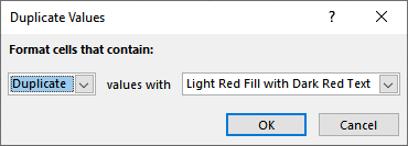
Figure 1. The Duplicate Values dialog box.
Be aware that the conditional formatting approach highlights all duplicates within your data, whereas the helper column approaches mentioned earlier flag only the second and subsequent occurrences of the data you are checking. Also, the conditional formatting approach checks only the first 255 characters of each cell.
ExcelTips is your source for cost-effective Microsoft Excel training. This tip (12843) applies to Microsoft Excel 2007, 2010, 2013, 2016, 2019, 2021, and Excel in Microsoft 365.

Program Successfully in Excel! This guide will provide you with all the information you need to automate any task in Excel and save time and effort. Learn how to extend Excel's functionality with VBA to create solutions not possible with the standard features. Includes latest information for Excel 2024 and Microsoft 365. Check out Mastering Excel VBA Programming today!
Sometimes getting the right thing to show up in a cell can be a bit tricky when working with dates. If you enter a year ...
Discover MoreWant a quick way to tell how may rows and columns you've selected? Here's what I do when I need to know that information.
Discover MoreDeleting rows or columns is easy when you use the shortcut described in this tip. Just select the rows or columns and ...
Discover MoreFREE SERVICE: Get tips like this every week in ExcelTips, a free productivity newsletter. Enter your address and click "Subscribe."
2022-02-19 22:07:26
Richard Hellenbrecht
Thank you Petyer and J. I think the Fuzzy Lookup will do the trick. Hopefully it works with Win 11 and MS365, but we'll see. Moving to a new PC right now, but I can't wait to try it. Thanks to all who replied.
2022-02-18 10:28:26
J. Woolley
@Richard Hellenbrecht
Have you tried Microsoft's Fuzzy Lookup Add-In for Excel? See
https://www.microsoft.com/en-us/download/details.aspx?id=15011
2022-02-18 10:10:10
Petyer Atherton
Richard Hellenbrecht
I would try to merge the files and work from there. If the fields do not agree in order and type you may be able to Get & Transform (Data tab) to order the columns but I'm not honestly sure. Then sort the data on Company names and that might be sufficient for you to identify duplicates.
I've written a couple of macros including the ISLIKE UDF that might help. You will not need the last name function
Sub Compare()
Dim r As Range, c2f As String, c As Range, _
nr As Long, counter As Long, i As Long, _
bIsLike As Boolean, s As String
Set r = Selection
nr = r.Rows.Count
For i = 1 To nr
counter = 0
c2f = "*" & LastName(r(i)) & "*"
For Each c In r
s = c
bIsLike = ISLIKE(s, c2f)
If bIsLike Then
counter = counter + 1
If counter > 1 Then c.Offset(0, 4) = "Duplicate"
End If
Next c
Next i
End Sub
Function ISLIKE(text As String, Pattern As String) As Boolean
If text Like Pattern Then ISLIKE = True _
Else ISLIKE = False
End Function
(see Figure 1 below)
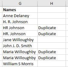
Figure 1.
2022-02-17 21:46:20
Richard Hellenbrecht
Re: Identifying Duplicates
Peter Atherton. I should have been more clear. I am not working with just first and last names. I am merging three separate database downloads into one file of about 16,000 records. Neither of these files have strong entry controls. They contain company names, not persons' names. A period, or lack of period in initial; spaces between initials, or no space; ", Inc." or just "Inc." cannot be queried.
The same company is interpreted differently under these circumstances. I'm looking for a "fuzzy" duplicate finder. After finding exact matches, about 3,000, I try phone numbers, then last names to weed out more, but its grueling. Ideas?
2022-02-17 10:01:34
Peter Atherton
Stephanie & Tomek
Any large number can only be shown in Excel as text, so the range must be pre-formatted as text. Writing a UDF does seem to work but if you want to have a list this macro will do it.
Sub Incre()
Dim startNumber, s1 As String, s2 As Long
Dim i As Long
startNumber = Range("a1")
s1 = Left(startNumber, 8)
s2 = Right(startNumber, Len(startNumber) - 8)
For i = 1 To 10
'Debug.Print s1 & s2 + i
Cells(i + 1, 1) = s1 & s2 + i
Next i
End Sub
2022-02-16 13:57:51
@Stephanie:
It seems that Excel cannot handle numbers with more than 15 significant digits. I you enter the *number* 1234567891234567, excel will change it to 1234567891234560 truncating digits after 15th.
If you enter that number into a cell formatted as text it will keep all digits. If you use such entry in an arithmetic calculation it will be truncated, e.g. if you have 1234567891234567 in the Cell A1 and in the cell A2 enter =A1+1 you will get 1234567891234560. (see Figure 1 below)
Note that in the picture below the cell 2 is formatted explicitly as number with 1 decimal, otherwise you may see 1.23457E+15, which hides the exact content.
Similar thing happens when you use conditional formatting for duplicates: even though the content of the cell is text, Excel sees that it looks as a number and treats it as a number hence truncating it to 15 significant digits. This happens even if you enter the number with a leading apostrophe to force it to be text and keep all digits.
Allen's first helper-column approach works for the situation you described, so this may be your best option. The second helper column approach does not work, as it uses a COUNTIF function and this triggers the "looks as a number - is a number" Excel logic.
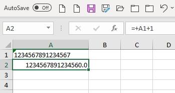
Figure 1.
2022-02-15 09:15:41
Sheryl Lucas
The conditional formatting tip rocks! Thank you, Allen!!!!
2022-02-14 09:38:55
Stephanie Hyder
You may want to add an exception to this statement..."Be aware that the conditional formatting approach highlights all duplicates within your data, whereas the helper column approaches mentioned earlier flag only the second and subsequent occurrences of the data you are checking. Also, the conditional formatting approach checks only the first 255 characters of each cell."
I consistently have numerical values flagged as duplicates using the conditional formatting approach because the first 15 characters are the same.
For example, these values all flag as duplicate even though the 16th character is different
1234567891234567
1234567891234568
1234567891234569
However, I did test the above values by replacing one character with a letter and Excel removed the "duplication" formatting. I believe the 255 character statement is accurate for cells containing alphabet characters.
If you know your data set has long numeric strings only, you may want to seriously consider a helper column, even if you only use one to investigate the duplicates identified by the conditional formatting.
I work with data sets that are thousands of lines long and often have this 15-character issue in the serial number column. I definitely use a helper column on the smaller subset of formatted "duplicates" to avoid the workbook from bogging down with non-essential formula calculations.
2022-02-14 05:49:57
Peter Atherton
Richard Hellenbrecht
A little more robust method than the lastName function would be to Add the first initial to the last name. But it would still fail with two brothers name William and Walter or a marrid couple named Chas and Cheryl.
Function CheckName(ByVal ref) As String
Dim p As Integer
p = InStrRev(ref, " ") + 1
CheckName = Mid(ref, 1, 1) & " " & Mid(ref, p, Len(ref))
End Function
Entered as =CheckName(A1)
(see Figure 1 below)
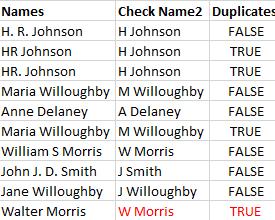
Figure 1.
2022-02-13 07:14:06
Peter Atherton
Richard Hellenbrecht
For poorly entered data as shown you need a helper column showing just the last names, then you can use Micky's formula. Here is a UDF for the last names.
Function LastName(ByVal ref) As String
Dim p As Integer
p = InStrRev(ref, " ") + 1
LastName = Mid(ref, p, Len(ref))
End Function
If you have not used UDFs before, right-click the sheet tab, select view code, Select Insert Module, paste in the code, & press Alt + Q to rteturn to sheet.
(see Figure 1 below)
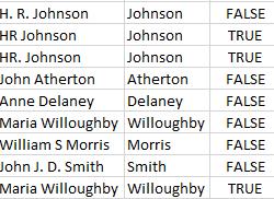
Figure 1. Last Names
2022-02-12 13:09:02
Richard Hellenbrecht
Duplicate identifier is very helpful for exact duplicates. But what about near-duplicates, such as H.R. Johnson vs HR Johnson or H. R. Johnson? Is there a function in Excel to do that?
2022-02-12 07:59:26
Michael (Micky) Avidan - MVP
As for the asked question - as per my opinion - there is no nee for a Helper-Column NOR a build-in Conditional-Formatting layout.
The use of C.F. leaning on the formula =COUNTIF(C$2:C2,C2)>1 is more than enough.
Got a version of Excel that uses the ribbon interface (Excel 2007 or later)? This site is for you! If you use an earlier version of Excel, visit our ExcelTips site focusing on the menu interface.
FREE SERVICE: Get tips like this every week in ExcelTips, a free productivity newsletter. Enter your address and click "Subscribe."
Copyright © 2026 Sharon Parq Associates, Inc.
Comments