Please Note: This article is written for users of the following Microsoft Excel versions: 2007, 2010, 2013, 2016, 2019, and 2021. If you are using an earlier version (Excel 2003 or earlier), this tip may not work for you. For a version of this tip written specifically for earlier versions of Excel, click here: Engineering Calculations.
Written by Allen Wyatt (last updated August 16, 2023)
This tip applies to Excel 2007, 2010, 2013, 2016, 2019, and 2021
In an engineering environment, it is not unusual to need to "normalize" numbers in some manner. For instance, you may need to show numeric values normalized to multiples of 10^3, such that 7340 is expressed as 7.34 and 73400 is expressed as 73.4.
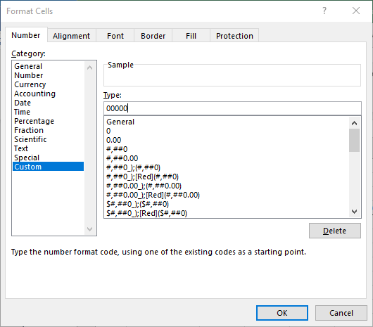
It is possible in Excel to use a custom number format to express information in scientific notation that will normalize the display of a number to a multiple of 10^3. To do this, you would follow these steps:

Figure 1. The Number tab of the Format Cells dialog box.
Now, when you enter a number such as 7340 into the cell, Excel displays it as 7.3E+3. Because of the way the cell format was entered, the portion after the E will always be a multiple of 3.
This is fine and good, but what if you want just the 7.3 in the cell, and then a metric prefix with a unit in an adjoining cell, such as kilograms? This is a bit more complex, but it can be done using formulas. For instance, let's assume you have your original number in cell A2, you wanted the normalized number in cell B2, and the metric prefix and unit name in cell C2. All you would need to do is enter the following formula in cell B2:
=IF(OR(A2>=1,A2<=-1),SIGN(A2)*(ABS(A2)/(10^(3*INT(LOG(ABS(A2))/3))))),
IF(A2=0,0,SIGN(A2)*(ABS(A2)*10^(-3*INT(LOG(ABS(A2))/3)))))
Assuming the units you are working with are an imaginary unit called a foo, in cell C2 you would use a different formula, as follows:
=IF(OR(A2>=1, A2<=-1),CHOOSE(INT(LOG(ABS(A2))/3)+1, "Foos", "Kilofoos",
"Megafoos", "Gigafoos", "Terafoos", "Petafoos", "Exafoos"),
IF(A2=0,"",CHOOSE(INT(-LOG(ABS(A2))/3)+1, "Millifoos", "Microfoos",
"Nanofoos", "Picofoos", "Femtofoos", "Attofoos")))
These formulas may seem a bit long, and they are. However, they will work for any number between approximately -9.99999E-18 to 9.99999E+20. For instance, if you put the number .000125 in cell A2, then cell B2 will contain 125 and cell C2 would contain Millifoos.
If you prefer to not use longer formulas such as these in your workbooks, you can develop a couple of VBA functions to do the trick. The following function, MySciNum, returns a normalized number. Thus, you would use =MySciNum(A2) in cell B2 to get the same results as noted above:
Function MySciNum(BaseNum As Double) As Double
    Select Case BaseNum
        Case Is >= 1
            While Abs(BaseNum) > 1000
                BaseNum = BaseNum / 1000
            Wend
        Case 0
            'Do nothing
        Case Else
            While Abs(BaseNum) < 1
                BaseNum = BaseNum * 1000
            Wend
    End Select
    MySciNum = BaseNum
End Function
This function only returns a number. To return the units with the appropriate metric prefix, you would use the following function. All you need to do is pass it the cell reference and the name of a single unit. For instance, you could use =MySciPre(A2, "foo"). The macro is as follows:
Function MySciPre(BaseNum As Double, Unit As String) As String
    Dim OrigNum As Double
    Dim Pref As Integer
    Dim Temp As String

    Pref = 0
    OrigNum = BaseNum
    Select Case BaseNum
        Case Is >= 1
            While Abs(BaseNum) > 1000
                BaseNum = BaseNum / 1000
                Pref = Pref + 1
            Wend
        Case 0
            Pref = 99
        Case Else
            While Abs(BaseNum) < 1
                BaseNum = BaseNum * 1000
                Pref = Pref - 1
            Wend
    End Select

    Select Case Pref
        Case -6
            Temp = "atto" & Unit
        Case -5
            Temp = "femto" & Unit
        Case -4
            Temp = "pico" & Unit
        Case -3
            Temp = "nano" & Unit
        Case -2
            Temp = "micro" & Unit
        Case -1
            Temp = "milli" & Unit
        Case 0
            Temp = Unit
        Case 1
            Temp = "kilo" & Unit
        Case 2
            Temp = "mega" & Unit
        Case 3
            Temp = "giga" & Unit
        Case 4
            Temp = "tera" & Unit
        Case 5
            Temp = "peta" & Unit
        Case 6
            Temp = "exa" & Unit
        Case Else
            Temp = ""
    End Select

    If Len(Temp) > 0 Then
        Temp = LCase(Temp)
        Temp = UCase(Left(Temp, 1)) & Mid(Temp, 2)
        If Abs(OrigNum) <> 1 Then Temp = Temp & "s"
    End If

    MySciPre = Temp
End Function
Note:
ExcelTips is your source for cost-effective Microsoft Excel training. This tip (12874) applies to Microsoft Excel 2007, 2010, 2013, 2016, 2019, and 2021. You can find a version of this tip for the older menu interface of Excel here: Engineering Calculations.

Program Successfully in Excel! This guide will provide you with all the information you need to automate any task in Excel and save time and effort. Learn how to extend Excel's functionality with VBA to create solutions not possible with the standard features. Includes latest information for Excel 2024 and Microsoft 365. Check out Mastering Excel VBA Programming today!
When sharing workbooks with others, you may find that the macros in those workbooks may not work as you expect. This tip ...
Discover MoreWhen creating macros, it is often necessary to change from one type of data to another. Here's how you can change from a ...
Discover MoreWhen creating an application in VBA for others to use, you might want a way for your VBA code to modify or delete other ...
Discover MoreFREE SERVICE: Get tips like this every week in ExcelTips, a free productivity newsletter. Enter your address and click "Subscribe."
2023-06-12 17:54:52
dox
Has no one noticed that "if you put the number .000125 in cell A2, then cell B2 will contain 125 and cell C2 would contain Millifoos" should read microfoos? (I'm not sure yet if this is an error in the equation or just a typo.)
Since this is Engineering, shouldn't we use "a, f, p, n, µ, m, k, M, G, T, P, E" symbols?
And I, as so many others, want my engineering notation with a specific number of significant digits. Although answered in the comments, this should be included in the article.
2021-09-28 10:18:03
Jeff Slotnick
thanks for the clear direction for setting engineering notation!
2021-07-16 13:29:10
Chris Fisichella
Thank you very much!
2020-09-03 06:47:44
Yali
If for example you have 0.00000000000419 or 4.19E-12 on cell C4 you can use this formula:
=C4*1000000000000&"ps"
It's a case by case basis but if all your numbers have the same unit then you can just use autofill. Hope it helps!
2019-07-29 12:08:17
Peter Atherton
Lars
When it is that important we can alway try a macro or UDF. We can't apply formatting with a function but, if you had a lot of numbers, we could write a procedure to change the format later.
Function N23Sig(ByVal ref As Range) As Double
Dim tmp As Double, L As Integer
If Len(ref) < 4 Then
N23Sig = Application.Round(ref / 1000, 2)
Exit Function
End If
tmp = ref / 1000
L = Len(tmp)
If L > 4 Then
N23Sig = Left(tmp, 4)
Else
N23Sig = tmp
End If
End Function
PS. You could write to Microsoft suggesting this option.
HTH
PPS. Actually, this formula works but I got it after writing the function. Moral; keep away from TEXT functions!
=LEFT(ROUND(I18/1000,2),4)*1
2019-07-29 01:56:37
Lars
Peter.
Thanks for your effort.
I've done something similar but, as you write, it's no longer numeric.
I cannot understand why Excel does not have the option "number significant digits".
2019-07-25 11:30:52
Peter Atherton
Lars
We can use the TEXT function to get what you want but if will convert is to text and you will lose the number. See if you can live with the following:
=IF(LEN(G2)=4,TEXT(ROUND(G2/1000,2),"0.00 10^3"),(ROUND(G2/1000,(LEN(G2)-4))))
[{Fig}]
2019-07-25 11:29:38
Peter Atherton
Lars
We can use the TEXT function to get what you want but if will convert is to text and you will lose the number. See if you can live with the following:
=IF(LEN(G2)=4,TEXT(ROUND(G2/1000,2),"0.00 10^3"),(ROUND(G2/1000,(LEN(G2)-4))))
[{Fig}]
2019-07-25 03:53:57
Lars
Peter.
Nice solution of 10^3.
My real question was how to get 3 significant digits without having to change number of decimals.
2019-07-24 12:05:59
Peter Atherton
Lars
Try this formula, with n in B2:
=IF(LEN(B2)=4,B2/1000,(ROUND(B2/1000,(LEN(B2)-4))))
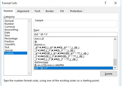
And use this custom Format as shown:
(see Figure 1 below)
You will need to increase the decimals for the second number

Figure 1. Custom Format "10^3"
2019-07-24 09:32:15
MIchael Armstrong
Beautiful; would have take me days to do that, if I hadn't given up altogether. Not looking forward to the day I have to deal with Exafoos.
2019-07-23 06:45:35
Lars
How do I accomplish "7340 is expressed as 7.34 10^3 and 73400 is expressed as 73.4 10^3", that is allways 3 significant digits, without using VBA.
Got a version of Excel that uses the ribbon interface (Excel 2007 or later)? This site is for you! If you use an earlier version of Excel, visit our ExcelTips site focusing on the menu interface.
FREE SERVICE: Get tips like this every week in ExcelTips, a free productivity newsletter. Enter your address and click "Subscribe."
Copyright © 2026 Sharon Parq Associates, Inc.
Comments