Highlighting an Entire Row for the Current Date

Ronald has a worksheet with 365 or 366 rows, one for each day. The date is in column B. Using conditional formatting he can highlight the current date, but Ronald wonders how he can highlight the whole row for the current date.

This is relatively easy to do, provided you know a trick in setting your conditional formatting rule. Let's say that you have your data in the range of A1:T367, with the first row being used for column headings. You need to select all the rows that may have dates in them. So, in this case you would either select the range A2:T367, or simply select rows 2 through 367. (Either selection will work just fine.) Now, follow these steps:

1. Make sure the Home tab of the ribbon is displayed.
2. Click the Conditional Formatting tool. Excel displays a series of choices.
3. Click New Rule. Excel displays the New Formatting Rule dialog box.
4. In the Select a Rule Type area at the top of the dialog box, choose Use a Formula to Determine Which Cells to Format. (See Figure 1.)



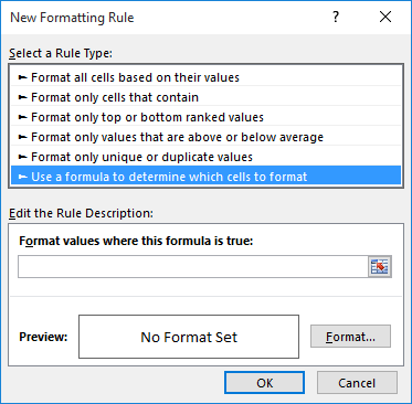
Figure 1. The New Formatting Rule dialog box.

5. In the formula space, enter the following formula:

     =$B2=TODAY()

6. Click on the Format button. Excel displays the Format Cells dialog box.
7. Use the controls in the dialog box to specify how you want your row formatted.
8. Click OK to close the Format Cells dialog box.
9. Click on OK to close the New Formatting Rule dialog box.

The "trick" I mentioned earlier is in step 5, when you define your formula. Remember that you started out by selecting a large range of cells or a large number of rows. That selection determines the cells to which the conditional formatting rule will be applied. However, the formula indicates that only the values in column B will be taken into consideration when evaluating the rule. This is the purpose of the dollar sign ($) it indicates an absolute column, one that doesn't change. Thus, all cells will be formatted when the formula is true, meaning that the date in column B is equal to today.

ExcelTips is your source for cost-effective Microsoft Excel training. This tip (13389) applies to Microsoft Excel 2007, 2010, 2013, 2016, 2019, 2021, and Excel in Microsoft 365.