Please Note: This article is written for users of the following Microsoft Excel versions: 2007, 2010, 2013, 2016, 2019, and 2021. If you are using an earlier version (Excel 2003 or earlier), this tip may not work for you. For a version of this tip written specifically for earlier versions of Excel, click here: Setting Up Custom AutoFiltering.
Written by Allen Wyatt (last updated July 8, 2023)
This tip applies to Excel 2007, 2010, 2013, 2016, 2019, and 2021
When are using Excel's AutoFiltering feature, you may want to display information in your list according to a custom set of criteria.
Excel makes this easy to do. All you need to do is the following:
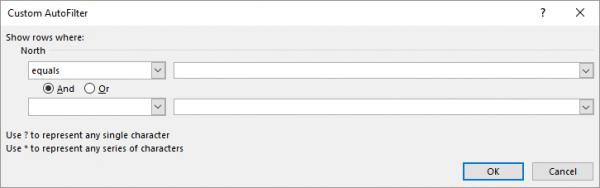
Figure 1. The Custom AutoFilter dialog box.
You can use the Custom AutoFilter dialog box to set any combination of criteria that you need. For instance, you can indicate that you want to see any values below, within, or above any given thresholds you desire. The filtering criteria will even work just fine with text values. For instance, you can cause Excel to display only records that are greater than AE. This means that anything beginning with AA through AE won't be displayed in the filtered list.
You should note that Excel also provides wildcard characters you can use to filter text values. These are the same wildcards you can use in specifying file names at the Windows command prompt. For instance, the question mark matches any single character, and the asterisk matches any number of characters. Thus, if you wanted to only display records that have the letter T in the third character position, you would use the equal sign operator (=) and a value of ??T*. This means the first two characters can be anything, the third character must be a T, and the rest can be anything.
ExcelTips is your source for cost-effective Microsoft Excel training. This tip (6711) applies to Microsoft Excel 2007, 2010, 2013, 2016, 2019, and 2021. You can find a version of this tip for the older menu interface of Excel here: Setting Up Custom AutoFiltering.

Professional Development Guidance! Four world-class developers offer start-to-finish guidance for building powerful, robust, and secure applications with Excel. The authors show how to consistently make the right design decisions and make the most of Excel's powerful features. Check out Professional Excel Development today!
When you have a column full of names, you may want to get a count of how many of those names are unique. You can make ...
Discover MoreExcel's AutoFilter tool is a great way to make a long list of items much more manageable. This tip explains how to set up ...
Discover MoreExcel has some built-in limits on what you can do with the program. When you run into those limits, it can be frustrating ...
Discover MoreFREE SERVICE: Get tips like this every week in ExcelTips, a free productivity newsletter. Enter your address and click "Subscribe."
2023-07-10 10:23:40
J. Woolley
My Excel Toolbox includes the following dynamic array function to list a worksheet's auto filters (Data > Filter):
=ListAutoFilters([Target],[SkipHeader])
It returns three rows (filter range, head cell's value, filter criteria) for Target's worksheet with one column for each filter plus an optional header column. Target can be a cell or range on any worksheet in an open workbook; if omitted, the formula's cell is assumed. If SkipHeader is FALSE (default), a header will be returned in the first column; otherwise, there will be no header column. You can swap rows and columns like this:
=TRANSPOSE(ListAutoFilters(...))
My Excel Toolbox's SpillArray function (described in UseSpillArray.pdf) simulates a dynamic array in older versions of Excel.
See https://sites.google.com/view/MyExcelToolbox
2023-07-10 07:49:58
Paul
Thanks J - this is exactly what I needed!
2023-07-09 12:22:40
J. Woolley
@Paul
If you have Excel 2019+, see the last example here: https://support.microsoft.com/en-us/office/filter-function-f4f7cb66-82eb-4767-8f7c-4877ad80c759
2023-07-08 11:52:16
Paul
Excel applies filters on multiple columns using AND logic. I would like to give my users the option to set filters on multiple columns using OR between the columns instead of the default AND behavior. Is there a way to do this?
Got a version of Excel that uses the ribbon interface (Excel 2007 or later)? This site is for you! If you use an earlier version of Excel, visit our ExcelTips site focusing on the menu interface.
FREE SERVICE: Get tips like this every week in ExcelTips, a free productivity newsletter. Enter your address and click "Subscribe."
Copyright © 2024 Sharon Parq Associates, Inc.
 Please Note:
This article is written for users of the following Microsoft Excel versions: 2007, 2010, 2013, 2016, 2019, and 2021. If you are using an earlier version (Excel 2003 or earlier), this tip may not work for you. For a version of this tip written specifically for earlier versions of Excel, click here:
Please Note:
This article is written for users of the following Microsoft Excel versions: 2007, 2010, 2013, 2016, 2019, and 2021. If you are using an earlier version (Excel 2003 or earlier), this tip may not work for you. For a version of this tip written specifically for earlier versions of Excel, click here:
Comments