Written by Allen Wyatt (last updated December 21, 2024)
This tip applies to Excel 2007, 2010, 2013, 2016, 2019, 2021, and Excel in Microsoft 365
Travis has a cell that, through a series of formulas, contains the upper-left corner of a 5 column by 20 row area that needs to be printed. For instance, if the cell contains $F$15, then the print area would be F15:J34, but if it contained $D$45, then the print area would be D45:H64. Travis wonders if it is possible to dynamically set the print area based on the contents of the cell, without using a macro.
Yes, there is a way you can set a dynamic print area without using a macro. Let's assume for the purposes of this tip that the calculated cell address is in A1. In preparation, you need to set up a print area:
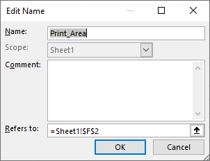
When you set a print area in this manner, Excel creates a named range called Print_Area. Whatever range it refers to is what will be printed when you choose to print. Since it is a named range, you can modify it in the Name Manager. Follow these steps to make the print area dynamic:

Figure 1. The Edit Name dialog box.
=OFFSET(INDIRECT(Sheet1!$A$1),,,20,5)
That's it. Your print area is now dynamic, dependent on the address stored in cell A1.
ExcelTips is your source for cost-effective Microsoft Excel training. This tip (13946) applies to Microsoft Excel 2007, 2010, 2013, 2016, 2019, 2021, and Excel in Microsoft 365.

Create Custom Apps with VBA! Discover how to extend the capabilities of Office 365 applications with VBA programming. Written in clear terms and understandable language, the book includes systematic tutorials and contains both intermediate and advanced content for experienced VB developers. Designed to be comprehensive, the book addresses not just one Office application, but the entire Office suite. Check out Mastering VBA for Microsoft Office 365 today!
Excel allows you to specify which portions of a worksheet should be printed when you send output to your printer. If you ...
Discover MoreMany people, when they print a worksheet, print the entire thing. You don't have to, however. You can specify that Excel ...
Discover MoreNeed to print more than one portion of your worksheet? If you use named ranges for the different ranges you want to ...
Discover MoreFREE SERVICE: Get tips like this every week in ExcelTips, a free productivity newsletter. Enter your address and click "Subscribe."
2024-12-21 13:22:01
Tomek
I like the solution presented in this tip (I suggested this approach in my reply to help-wanted, but I probably wasn’t the only one). It is relatively simple, does what Travis wanted, and does not “contaminate” the spreadsheet with helper cells. What Allen did not mention was that the address of the cell A1 in the formula must be entered as an absolute address, i.e., Sheet1! $A$1; if it is entered as the relative address the Print_Area is not set properly, and the approach does not work (why? – I don’t know).
I also suggested another approach, that may not be as elegant, but potentially may have additional advantages. The steps are as follows:
1. Select a 20-rows by 5-columns range somewhere on the sheet, where it would not interfere with your data. Set the Print Area to that range.
2. In the top left corner of that print area enter =OFFSET(INDIRECT($A$1),0,0,20,5). This formula will spill and populate Print_Area with a copy of what you want to print, and when you print the sheet, it is what will be printed. As in the tip, I assume that the calculated cell address is in A1.
3. If using an older version of Excel that does not automatically spill into Array, you will need to enter the above formula as an Array Formula (Ctrl+Shift+<ENTER>) covering the whole Print_Area range.
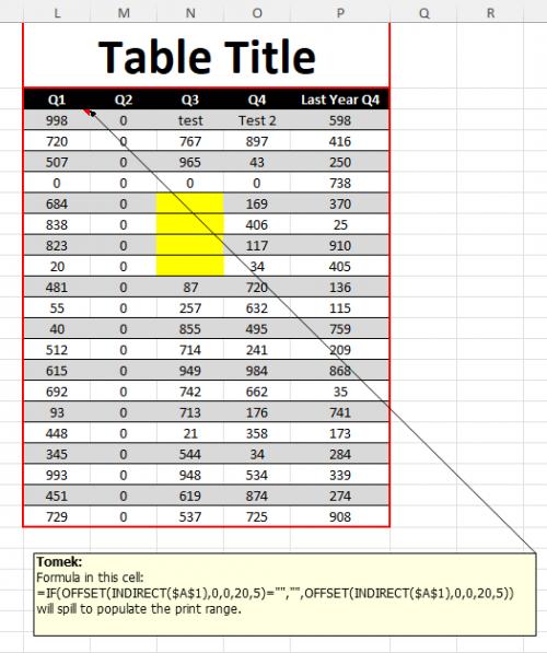
The benefit of this approach is that you can format the data that is in the Print_Area any way you want, independently of the format of original data. Additionally, you can add rows above to add column labels and possibly the title, and add a column to the left for row labels. Those do not have to be static but can also depend on the content of A1. If you add rows and columns, obviously you will need to adjust the print area to include them as well.
There is one disadvantage of this approach: if any of the original cells are blank, they will show in the print area as zeros, probably not what you would want. It can be easily overcome by slight modification of the formula entered in step 2 as follows:
=IF(OFFSET(INDIRECT($A$1),0,0,20,5)="","",OFFSET(INDIRECT($A$1),0,0,20,5))
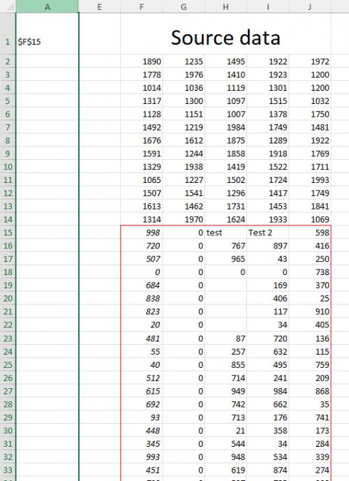
See screenshots of my test workbook (see Figure 1 below) (see Figure 2 below)

Figure 1. Source Data

Figure 2. Formatted Print Area
Got a version of Excel that uses the ribbon interface (Excel 2007 or later)? This site is for you! If you use an earlier version of Excel, visit our ExcelTips site focusing on the menu interface.
FREE SERVICE: Get tips like this every week in ExcelTips, a free productivity newsletter. Enter your address and click "Subscribe."
Copyright © 2026 Sharon Parq Associates, Inc.
Comments