Weighted Averages in a PivotTable

A good example of how to use calculated fields is for summarizing data differently than you can normally summarize it with a PivotTable. When you create a PivotTable, you can use several different functions to summarize the data that is displayed. For instance, you can create an average of data in a particular field. What if you want to create a weighted average, however? Excel doesn't provide a function that automatically allows you to do this.

When you have special needs for summations—like weighted averages—the easiest way to achieve your goal is to add an additional column in the source data as an intermediate calculation, and then add a calculated field to the actual PivotTable.

For example, you could add a "WeightedValue" column to your source data. The formula in the column should multiply the weight times the value to be weighted. This means that if your weight is in column C and your value to be weighted is in column D, your formula in the WeightedValue column would simply be like =C2*D2. This formula will be copied down the entire column for all the rows of the data.

You are now ready to create your PivotTable, which you should do as normal with one exception: you need to create a Calculated Field. Follow these steps:

1. Select any of the cells in the PivotTable.
2. On the ribbon, make sure the Options tab (Excel 2007 and Excel 2010) or the Analyze tab (Excel 2013 and Excel 2016) is displayed.
3. Display the Insert Calculated Field dialog box. (If you are using Excel 2007, in the Tools group click the Formulas tool and then choose Calculated Field. If you are using Excel 2010 or a later version, in the Calculations group click the Fields, Items & Sets tool and then choose Calculated Field.) (See Figure 1.)



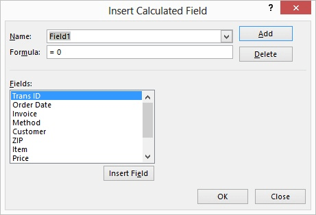
Figure 1. The Insert Calculated Field dialog box.

4. In the Name box, enter a name for your new field.
5. In the Formula box, enter the formula you want used for your weighted average, such as =WeightedValue/Weight. (You use field names in the formula; you can select them from the field list at the bottom of the Insert Calculated Field dialog box.)
6. Click OK.

Your calculated field is now inserted, and you can use the regular summation functions to display a sum of the calculated field; this is your weighted average.

Since there are many different ways that weighted averages can be calculated, it should go without saying that you can modify the formulas and steps presented here to reflect exactly what you need done with your data.

ExcelTips is your source for cost-effective Microsoft Excel training. This tip (7129) applies to Microsoft Excel 2007, 2010, 2013, and 2016. You can find a version of this tip for the older menu interface of Excel here: Weighted Averages in a PivotTable.