Highlighting Pattern Violations

Steve has a worksheet that contains over ten thousand rows, with each cell in column A containing a file name. These names need to follow two rules, and Steve needs to discover which names violate either of the rules. If a file name contains a dash, it must also have a single space before and after the dash. The second rule is that if the name contains a comma, there must be no space before it but a single space after it. Steve wonders how he can highlight cells that violate either (or both) of these rules.

Anytime someone mentions that they want to "highlight" something in a worksheet, most people think of using conditional formatting. This instance is no exception; you could easily use conditional formatting to highlight the pattern violations. The key to developing the conditional formatting rule is to come up with a formula that returns True if the pattern is violated. This formula checks for both violations:

=OR(ISNUMBER(FIND("-",SUBSTITUTE(A1," - ",""))),
ISNUMBER(FIND(",",SUBSTITUTE(A1,", ",""))),
ISNUMBER(FIND(" ,",A1)))

I've broken the formula to three lines here, but it should be considered one complete formula. The formula removes the correct patterns (space, dash, space and comma, space) from the filename, and then checks to see if either a dash or comma remains in the filename. If one does remain, then the formula returns True.

You can set up a conditional formatting rule to use the formula in this manner:

1. Select the cells that contain all the filenames you want checked.
2. With the Home tab of the ribbon displayed, click the Conditional Formatting option in the Styles group. Excel displays a palette of options related to conditional formatting.
3. Choose Highlight Cells Rules and then choose More Rules from the resulting submenu. Excel displays the New Formatting Rule dialog box. (See Figure 1.)



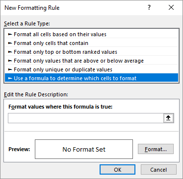
Figure 1. The New Formatting Rule dialog box.

4. In the Select a Rule Type area at the top of the dialog box, choose Use a Formula to Determine Which Cells to Format.
5. In the Format Values Where This Formula Is True box, enter the long formula already discussed.
6. Click Format to display the Format Cells dialog box.
7. Using the controls in the dialog box, specify a format that you want used to highlight the cells that violate your pattern.
8. Click OK to dismiss the Format Cells dialog box. The formatting you specified in step 7 should now appear in the preview area for the rule.
9. Click OK.

If the cells you selected in step 1 did not begin with cell A1, then you'll need to modify the formula used in step 5 to reflect your beginning cell. (All three instances of A1 in the formula would need to be changed to reference your beginning cell.)

There are two big "gotchas" in using this formula in your conditional formatting rule. First, it doesn't detect double spaces. So, for instance, if the filename contained "space, space, dash, space," that would be violation of the pattern. However, the SUBSTITUTE function in the formula would remove the "space, dash, space," leaving the extra space in the resulting string. This single space would not be detected as a violation of the pattern, even though it is.

The solution to this would be a much longer formula or bypassing the conditional formatting route altogether and starting to use helper columns. This feeds right into the second "gotcha," and it is a big one: If you apply conditional formatting (or add helper columns containing formulas) to ten thousand rows, you will notice a marked increase in how long it takes to recalculate your worksheet. There is no way around this when you start adding so many formulas to the worksheet.

For this reason, you may find it more appropriate to develop a macro that highlights the cells. The macro could then be run manually when you want to check the patterns, which means your normal worksheet recalculation is not slowed down.

The following macro is designed to be run on a selected range of cells. It checks to make sure that there are not two spaces before a dash, two spaces after a dash, one space before a comma, or two spaces after a comma. It then removes any correctly patterened dashes and commas from the filename and checks to see if any dashes or commas remain. If a violation of any of these conditions is noted, then the cell is formatted with yellow.

Sub CheckFilenames1()
    Dim bBad As Boolean
    Dim c As Range
    Dim sTemp1 As String
    Dim sTemp2 As String

    For Each c In Selection
        bBad = False
        sTemp1 = c.Text

        If Instr(sTemp1, "  -") > 0 Then bBad = True
        If Instr(sTemp1, "-  ") > 0 Then bBad = True
        If Instr(sTemp1, " ,") > 0 Then bBad = True
        If Instr(sTemp1, ",  ") > 0 Then bBad = True
        sTemp2 = Replace(sTemp1, " - ", "")
        If Instr(sTemp2, "-") > 0 Then bBad = True
        sTemp2 = Replace(sTemp1, ", ", "")
        If Instr(sTemp2, ",") > 0 Then bBad = True

        If bBad Then
            c.Interior.Color = vbYellow
        Else
            c.Interior.Color = xlColorIndexNone
        End If
    Next c
End Sub

The macro may take a while to run but, again, it only needs to be run when you want to check the fielnames. If you don't want the macro to "mess up" the cell formatting, then you may want a version that inserts some text in the column to the right of any filenames that violate your desired pattern.

Sub CheckFilenames2()
    Dim bBad As Boolean
    Dim c As Range
    Dim sTemp1 As String
    Dim sTemp2 As String

    For Each c In Selection
        bBad = False
        sTemp1 = c.Text

        If InStr(sTemp1, "  -") > 0 Then bBad = True
        If InStr(sTemp1, "-  ") > 0 Then bBad = True
        If InStr(sTemp1, " ,") > 0 Then bBad = True
        If InStr(sTemp1, ",  ") > 0 Then bBad = True
        sTemp2 = Replace(sTemp1, " - ", "")
        If InStr(sTemp2, "-") > 0 Then bBad = True
        sTemp2 = Replace(sTemp1, ", ", "")
        If InStr(sTemp2, ",") > 0 Then bBad = True

        If bBad Then c.Offset(0, 1) = "BAD"
    Next c
End Sub

When run, this variation of the macro inserts the text "BAD" in the cell to the right of improperly patterend filenames. You can then use the filtering capabilities of Excel to display only those rows that contain the text.

Of course, you may want to take this all just a step further and allow the macro to modify any incorrectly formatted filenames. The following macro does its work on whatever cells you've selected. It ensures that each dash is surrounded by a single space and that each comma is followed only by a single space.

Sub FixFilenames()
    Dim myArry() As String
    Dim sTemp As String
    Dim c As Range
    Dim s As Variant

    For Each c In Selection
        myArry = Split(c, "-")
        sTemp = ""
        For Each s In myArry
            If sTemp > "" Then
                sTemp = sTemp & " - " & Trim(s)
            Else
                sTemp = Trim(s)
            End If
        Next s
        myArry = Split(sTemp, ",")
        sTemp = ""
        For Each s In myArry
            If sTemp > "" Then
                sTemp = sTemp & ", " & Trim(s)
            Else
                sTemp = Trim(s)
            End If
        Next s
        c = sTemp
    Next c
End Sub

ExcelTips is your source for cost-effective Microsoft Excel training. This tip (3015) applies to Microsoft Excel 2007, 2010, 2013, 2016, 2019, Excel in Microsoft 365, and 2021.