Please Note: This article is written for users of the following Microsoft Excel versions: 2007, 2010, 2013, 2016, 2019, and 2021. If you are using an earlier version (Excel 2003 or earlier), this tip may not work for you. For a version of this tip written specifically for earlier versions of Excel, click here: Importing Custom Lists.
Written by Allen Wyatt (last updated December 11, 2021)
This tip applies to Excel 2007, 2010, 2013, 2016, 2019, and 2021
Custom lists are a rather esoteric Excel feature that allows you to specify ordered lists of information for virtually any purpose. For instance, a list might include a series of classes or workshops, or it might include a series of employee names. Custom lists can be used when sorting data tables, and they can be used by the AutoFill feature.
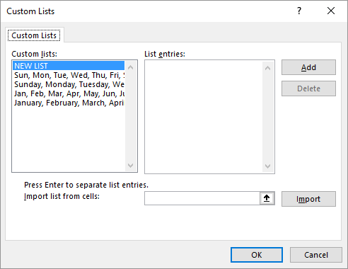
How you create a custom list from scratch has been covered in other issues of ExcelTips. Rather than creating a list from scratch, however, you might find it easier to import a list from a series of cells already in your worksheet. Follow these steps:

Figure 1. The Custom Lists dialog box.
You can now use the custom list as you would any other custom list in Excel.
ExcelTips is your source for cost-effective Microsoft Excel training. This tip (6243) applies to Microsoft Excel 2007, 2010, 2013, 2016, 2019, and 2021. You can find a version of this tip for the older menu interface of Excel here: Importing Custom Lists.

Professional Development Guidance! Four world-class developers offer start-to-finish guidance for building powerful, robust, and secure applications with Excel. The authors show how to consistently make the right design decisions and make the most of Excel's powerful features. Check out Professional Excel Development today!
Sorting ZIP Codes can be painless, provided all the codes are formatted the same. Here's how to do the sorting if you ...
Discover MoreSorting information in Excel is a common task. Sorting information that isn't in the primary order that you need can be a ...
Discover MoreWhen you sort your data, you should always check to see if the sort was done correctly. What if sorting messes up ...
Discover MoreFREE SERVICE: Get tips like this every week in ExcelTips, a free productivity newsletter. Enter your address and click "Subscribe."
2021-12-11 10:30:19
J. Woolley
My Excel Toolbox includes the dynamic array function ListCustomLists(), which simply lists all of Excel's Custom Lists (built-in plus user-defined) as an array with 1 column and N rows. You can use it like this:
=ListCustomLists()
In older versions of Excel you can use it with the SpillArray function like this:
=SpillArray(ListCustomLists())
See https://sites.google.com/view/MyExcelToolbox/
Got a version of Excel that uses the ribbon interface (Excel 2007 or later)? This site is for you! If you use an earlier version of Excel, visit our ExcelTips site focusing on the menu interface.
FREE SERVICE: Get tips like this every week in ExcelTips, a free productivity newsletter. Enter your address and click "Subscribe."
Copyright © 2026 Sharon Parq Associates, Inc.
Comments