Please Note: This article is written for users of the following Microsoft Excel versions: 2007, 2010, 2013, 2016, 2019, 2021, 2024, and Excel in Microsoft 365. If you are using an earlier version (Excel 2003 or earlier), this tip may not work for you. For a version of this tip written specifically for earlier versions of Excel, click here: Displaying a Hidden First Column.
Excel makes it easy to hide and unhide columns. What isn't so easy is displaying a hidden column if that column is the left-most column in the worksheet. For instance, if you hide column A, Excel will dutifully follow out your instructions. If you later want to unhide column A, the solution isn't so obvious.
To unhide the left-most columns of a worksheet when they are hidden, follow these steps:
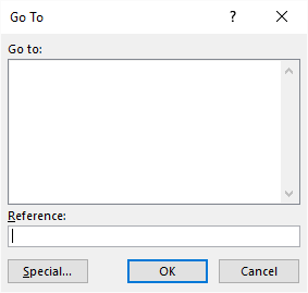
Figure 1. The Go To dialog box.
Another way to display the first column is to click on the header for column B, and then drag the mouse to the left. If you release the mouse button when the pointer is over the gray block that marks the intersection of the row and column headers (the blank gray block just above the row headers), then column B and everything to its left, including the hidden column A, are selected. You can then display the Home tab of the ribbon and click Format | Hide & Unhide | Unhide Columns.
A third method is even niftier, provided you have a good eye and a steady mouse pointer. If you move your mouse pointer into the column header area, and then slowly move it to the left, you notice that it turns into a double-headed arrow with a blank spot in the middle as you position the pointer over the small area immediately to the left of the column B header. This double-headed arrow is a bit difficult to describe; it looks most closely like the double-headed arrow that appears when you position the pointer over the dividing line between column headers. It is different, however, because instead of a black line dividing the double arrows, there are two black lines with a gap between them.
When your mouse pointer changes to this special double-headed arrow, all you have to do is right-click and choose Unhide. Your previously missing column A magically reappears.
ExcelTips is your source for cost-effective Microsoft Excel training. This tip (9012) applies to Microsoft Excel 2007, 2010, 2013, 2016, 2019, 2021, 2024, and Excel in Microsoft 365. You can find a version of this tip for the older menu interface of Excel here: Displaying a Hidden First Column.

Excel Smarts for Beginners! Featuring the friendly and trusted For Dummies style, this popular guide shows beginners how to get up and running with Excel while also helping more experienced users get comfortable with the newest features. Check out Excel 2019 For Dummies today!
We all expect the keyboard keys to operate as normal, and when they don't, it can be bothersome. Geraldine had such a ...
Discover MoreWhen you select a range of cells (particularly if it is a large range of cells), you may not be quite sure if you've ...
Discover MoreWant to keep track of various rows in a data table through the use of record numbers? Here are some options and ...
Discover MoreFREE SERVICE: Get tips like this every week in ExcelTips, a free productivity newsletter. Enter your address and click "Subscribe."
2025-09-27 08:47:25
Alex Blakenburg
I find the quickest way is to use the method 2 selection process ie select Column B using the mouse then drag left but then to just slightly adjust column B's size using the mouse which will make Column A the same size (unhiding it).
For method 1 using Go To, instead of using the Go To function dialogue box simply type A1 into Name Box in the top left corner just above A1 and hit enter. Then follow the instructions for method 1.
Got a version of Excel that uses the ribbon interface (Excel 2007 or later)? This site is for you! If you use an earlier version of Excel, visit our ExcelTips site focusing on the menu interface.
FREE SERVICE: Get tips like this every week in ExcelTips, a free productivity newsletter. Enter your address and click "Subscribe."
Copyright © 2026 Sharon Parq Associates, Inc.
 Please Note:
This article is written for users of the following Microsoft Excel versions: 2007, 2010, 2013, 2016, 2019, 2021, 2024, and Excel in Microsoft 365. If you are using an earlier version (Excel 2003 or earlier), this tip may not work for you. For a version of this tip written specifically for earlier versions of Excel, click here:
Please Note:
This article is written for users of the following Microsoft Excel versions: 2007, 2010, 2013, 2016, 2019, 2021, 2024, and Excel in Microsoft 365. If you are using an earlier version (Excel 2003 or earlier), this tip may not work for you. For a version of this tip written specifically for earlier versions of Excel, click here:
Comments