Mark knows he can use data validation to create a drop-down list. What he doesn't know is how to use the drop-down list in conjunction with the HYPERLINK function so the user can jump to a particular worksheet. In other words, they pick something in the drop-down list, then click on a link that says "Go to Report," and then the report they selected in the drop-down list is displayed. Mark wonders if there is a way to represent the report's worksheet (the target) in the drop-down list, as well as the name displayed in the drop-down list.
For Mark's purposes, I'm going to assume that the reports are contained on other worksheets in the current workbook. In that case, it would be good to define a small table that contains three columns. The first column contains the text you want in the validation list, perhaps the name of the reports. The second column is the name of the target worksheet containing the report, and the third column is the target cell within the worksheet. (See Figure 1.)
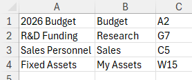
Figure 1. Setting up table information.
Notice that the table doesn't really need any column headings. I will, however, select the cells and give them a name. In this case, I'll use the name JumpTable. Using three columns in the table allows flexibility in specifying destination worksheets and cells. In fact, over time you can make any changes in the table desired, and your hyperlink will still work just fine.
Speaking of the hyperlink, the next step is to use data validation to set up a drop-down list. Select cell F1 and then, on the Data tab of the ribbon, click the Data Validation tool. Excel displays the Data Validation dialog box. Using the Allow drop-down list, choose List, and then enter this formula in the Source box:
=INDEX(JumpTable,0,1)
Click OK, and your drop-down list, in cell F1, is now populated with the values in the first column of the JumpTable range. Now you can combine this selection with the HYPERLINK function in the following manner:
=HYPERLINK("#"&TEXTJOIN("!",, XLOOKUP(F1, CHOOSECOLS(JumpTable,1), CHOOSECOLS(JumpTable,{2,3}))),"Go to Report")
This is a long formula, but it works because the TEXTJOIN function returns a combination of cells from the second and third columns of JumpTable based on a match in the first column. The way the formula is set up assumes that the worksheet name (in the second column) is only a single word. If the names contained in the second column contain spaces, then you'll want to modify the formula to add apostrophes around what is pulled from the second column:
=HYPERLINK(LET(r, XLOOKUP(F1, CHOOSECOLS(JumpTable,1), CHOOSECOLS(JumpTable,{2,3})), "#'" & INDEX(r,1,1) & "'!" & INDEX(r,1,2)),"Go to Report")
These formulas, though, will only work if you are using Excel 2021, Excel 2024, or Microsoft 365. If you are using an earlier version of the program, then you'll need to rely on older lookup functions:
=HYPERLINK("#" & IFERROR("#'" & VLOOKUP(F1,JumpTable,2,FALSE) & "'!" & VLOOKUP(F1,JumpTable,3,FALSE),""),"Go to Report")
ExcelTips is your source for cost-effective Microsoft Excel training. This tip (9424) applies to Microsoft Excel 2007, 2010, 2013, 2016, 2019, 2021, 2024, and Excel in Microsoft 365.

Solve Real Business Problems Master business modeling and analysis techniques with Excel and transform data into bottom-line results. This hands-on, scenario-focused guide shows you how to use the latest Excel tools to integrate data from multiple tables. Check out Microsoft Excel Data Analysis and Business Modeling today!
Data Validation is a great tool in Excel for making sure that whatever is entered in a cell matches your specific ...
Discover MoreWhen entering data in a worksheet, you may want to exercise some degree of control on the values that can be entered. ...
Discover MoreIf you want to make sure that only unique values are entered in a particular column, you can use the data validation ...
Discover MoreFREE SERVICE: Get tips like this every week in ExcelTips, a free productivity newsletter. Enter your address and click "Subscribe."
2025-11-18 18:44:17
Tomek
Gonzonator1982:
Thank you for your reply. I did not know that and there is no mention of this in the Microsoft help for the HYPERLINK function in Excel.
So I learned something new. And I thought I knew Excel - I have been using it for about 30 years.
2025-11-18 12:21:15
Gonzonator1982
Tomek, the Hash "#" tells the hyperlink formula to look inside the document for the hyperlink; without it, the hyperlink looks out to the web by default.
2025-11-16 16:35:44
Tomek
As I mentioned in my earlier comment, both the solution from Allen's tip, and my alternate macro-based approach may not properly display the requested report. If the range covering a particular report is away from left and/or top of the sheet, selecting the cell/range may display it far to the right/down with large portion of it hidden outside the visible part of the sheet. To avoid this, for the hyperlink solution, you can add a simple macro to each target sheet code:
Private Sub Worksheet_Activate()
Application.Goto Selection, Scroll:=True
End Sub
When the hyperlink is clicked, it will select the desired range on the target. Upon activating the target sheet, the screen will scroll to display the active cell in the top corner. And yes, you can pass a range of cells via hyperlink, not only a single cell. (see Figure 1 below) The limitation of this is that the report cannot be on the same sheet as the hyperlink, as this sheet is already active.
For the macro solution a slight modification will do the same. To make it more user friendly, I added the second window, in which the report will be displayed. So you will have two windows for the same file, one for the Table of Contents, and one for the report. Closing the second window after report is reviewed/printed will simply get you back to the Table of Contents.
As I said in my earlier comment, the macro approach saves you some clicks - only two are required for selecting from the drop-down list vs. four for the hyperlink approach. As I always say, there are many ways to skin a catfish (not a cat - I love cats), but some are better than others.
=========
Private Sub Worksheet_Change(ByVal Target As Range)
If Not Intersect(Target, Range("F1")) Is Nothing Then
ActiveWindow.NewWindow
sht = Range("G1").Value
cel = Range("H1").Value
Sheets(sht).Activate
ActiveSheet.Range(cel).Select
Application.Goto , True
End If
End Sub
====================
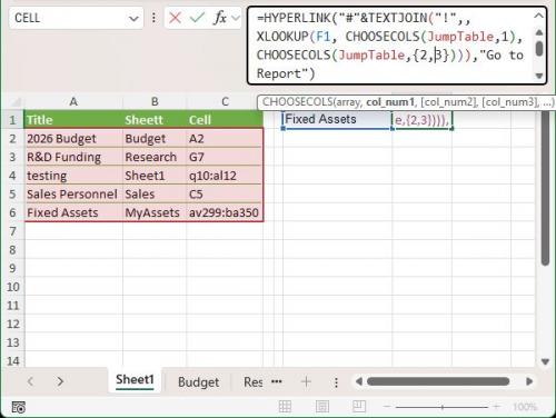
Figure 1.
2025-11-16 11:22:01
Tomek
@Peter
Your formula does not work
2025-11-16 00:55:36
Peter
I have used a jump table similar to this just using a macro, but found that if the target worksheet was edited the target cell often moved. To avoid ending up in the wrong cell, taking the last row of the example, I would refer to the target cell with the following formula in column C
=CELL("address",'My Assets'W15).
2025-11-15 23:03:14
Tomek
Further to my earlier comment:
You may not need to go to a specific target cell, just activate the sheet with the requested report.
In such case you can omit the entry in the cell H1, as well as two lines of the code making it simpler:
Private Sub Worksheet_Change(ByVal Target As Range)
If Not Intersect(Target, Range("F1")) Is Nothing Then
sht = Range("G1").Value
Sheets(sht).Activate
End If
End Sub
=================
In any case you may want to make sure that the relevant area of sheet that opens is properly positioned in the Excel Window; just selecting a particular cell does not necessarily position it in the upper left corner of the window. This applies also to the hyperlink method. How to get the proper view of the sheet with the report when it opens is a whole different story, and may be a subject of a future tip, if Allen agrees.
2025-11-15 22:43:38
Tomek
The method proposed in the tip works well and is exactly what Mark asked for, but it requires four or three clicks: select the cell with the multiple choice (unless already selected), click on the down arrow, select one of options from the drop-down list, then click the hyperlink in another cell. I think the last click is not necessary, hence the use of the hyperlink is also not necessary. On the other hand, my suggestion is to use a macro that some users may not not like or even be able to do (company policies).
I suggest the macro be triggered by a change in the cell with the drop-down list.
The setup is the same as in the tip, up to the point where the validation list is created in the cell F1.
Instead of creating a hyperlink in a nearby cell, use VLOOKUP based on JumpTable to get the sheet name and the target cell into the neighbouring cells G1 and H1, respectively:
=VLOOKUP(F1,JumpTable,2,FALSE)
=VLOOKUP(F1,JumpTable,3,FALSE)
(see Figure 1 below)
You could also use XLOOKUP for this purpose. Please note that for simplicity I made sure that sheet names have no spaces.
Once you have all this in place add the following macro to your "Table of Contents" sheet code:
Private Sub Worksheet_Change(ByVal Target As Range)
If Not Intersect(Target, Range("F1")) Is Nothing Then
sht = Range("G1").Value
cel = Range("H1").Value
Sheets(sht).Activate
ActiveSheet.Range(cel).Select
End If
End Sub
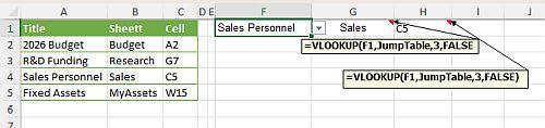
Figure 1.
2025-11-15 16:39:21
Tomek
What is the purpose of the "#" in the formula:
=HYPERLINK("#"&TEXTJOIN("!",, XLOOKUP(F1, CHOOSECOLS(JumpTable,1), CHOOSECOLS(JumpTable,{2,3}))),"Go to Report")
I know it is important, because it does not work without it, but I have no idea why.
Got a version of Excel that uses the ribbon interface (Excel 2007 or later)? This site is for you! If you use an earlier version of Excel, visit our ExcelTips site focusing on the menu interface.
FREE SERVICE: Get tips like this every week in ExcelTips, a free productivity newsletter. Enter your address and click "Subscribe."
Copyright © 2026 Sharon Parq Associates, Inc.
Comments