Please Note: This article is written for users of the following Microsoft Excel versions: 2007, 2010, 2013, 2016, 2019, and 2021. If you are using an earlier version (Excel 2003 or earlier), this tip may not work for you. For a version of this tip written specifically for earlier versions of Excel, click here: Using a Numeric Portion of a Cell in a Formula.
Rita described a problem where she is provided information, in an Excel worksheet, that combines both numbers and alphabetic characters in a cell. In particular, a cell may contain "3.5 V", which means that 3.5 hours of vacation time was taken. (The character at the end of the cell could change, depending on the type of hours the entry represented.) Rita wondered if it was possible to still use the data in a formula in some way.
Yes, it is possible, and there are several ways to approach the issue. The easiest way (and cleanest) would be to simply move the alphabetic characters to their own column. Assuming that the entries will always consist of a number, followed by a space, followed by the characters, you can do the "splitting" this way:
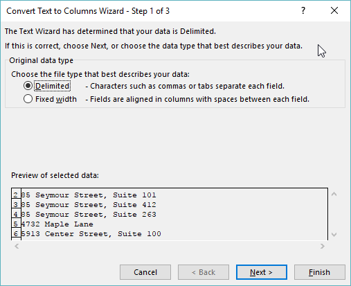
Figure 1. The first step of the Convert Text to Columns Wizard.
Word splits the entries into two columns, with the numbers in the leftmost column and the alphabetic characters in the right. You can then use any regular math functions on the numeric values that you desire.
If it is not feasible to separate the data into columns (perhaps your company doesn't allow such a division, or it may cause problems with those later using the worksheet), then you can approach the problem in a couple of other ways.
First, you could use the following formula on individual cells:
=VALUE(LEFT(A3,LEN(A3)-2))
The LEFT function is used to strip off the two rightmost characters (the space and the letter) of whatever is in cell A3, and then the VALUE function converts the result to a number. You can then use this result as you would any other numeric value.
If you want to simply sum the column containing your entries, you could use an array formula. Enter the following in a cell:
=SUM(VALUE(LEFT(A3:A21,LEN(A3:A21)-2)))
Make sure you actually enter the formula by pressing Shift+Ctrl+Enter. Because this is an array formula, the LEFT and VALUE functions are applied to each cell in the range A3:A21 individually, and then summed using the SUM function.
ExcelTips is your source for cost-effective Microsoft Excel training. This tip (10229) applies to Microsoft Excel 2007, 2010, 2013, 2016, 2019, and 2021. You can find a version of this tip for the older menu interface of Excel here: Using a Numeric Portion of a Cell in a Formula.

Solve Real Business Problems Master business modeling and analysis techniques with Excel and transform data into bottom-line results. This hands-on, scenario-focused guide shows you how to use the latest Excel tools to integrate data from multiple tables. Check out Microsoft Excel Data Analysis and Business Modeling today!
Creating math formulas is a particular strong point of Excel. Not all the functions that you may need are built directly ...
Discover MoreExcel provides a variety of tools that allow you to perform operations on your data based upon the characteristics of ...
Discover MoreDo you need to generate strings of random characters? The ideas presented in this tip will help you do it in a hurry.
Discover MoreFREE SERVICE: Get tips like this every week in ExcelTips, a free productivity newsletter. Enter your address and click "Subscribe."
2021-08-12 11:01:14
J. Woolley
@Lance
If your scenario includes the condition that both cells contain a constant value (not a formula), then you can use the following method.
Right-click on Sheet1's tab and pick View Code, then put this VBA in that worksheet's code frame:
Private Sub Worksheet_Change(ByVal Target As Range)
Const ThisCell = "$A$1", ThatCell = "$C$1", ThatSheet = "Sheet2"
If Target.Address = ThisCell Then
Application.EnableEvents = False
Worksheets(ThatSheet).Range(ThatCell) = Target
Application.EnableEvents = True
End If
End Sub
Right-click on Sheet2's tab and pick View Code, then put this VBA in that worksheet's code frame:
Private Sub Worksheet_Change(ByVal Target As Range)
Const ThisCell = "$C$1", ThatCell = "$A$1", ThatSheet = "Sheet1"
If Target.Address = ThisCell Then
Application.EnableEvents = False
Worksheets(ThatSheet).Range(ThatCell) = Target
Application.EnableEvents = True
End If
End Sub
Adjust ThisCell, ThatCell, and ThatSheet if necessary, but the cell address values must be absolute (like $A$1, not A1).
2021-08-12 04:29:53
Peter Atherton
Type = then point to the target cell and you get this: =Sheet2!C2; you could also reference a rane of cells e.g. =SUM(sheet2!C2:C20)
2021-08-11 22:21:53
Lance
Hello,
I love reading the weekly Excel Tips and have a question that I think is not possible but would like to pose this question to the experts. Is there a way to link a cell, say A1, in a worksheet, say Sheet1, with a cell, say C1, in a different worksheet, say Sheet2, in the same workbook so that no matter which cell you change the value in, the other will also change?
Thank you for your time
Got a version of Excel that uses the ribbon interface (Excel 2007 or later)? This site is for you! If you use an earlier version of Excel, visit our ExcelTips site focusing on the menu interface.
FREE SERVICE: Get tips like this every week in ExcelTips, a free productivity newsletter. Enter your address and click "Subscribe."
Copyright © 2026 Sharon Parq Associates, Inc.
 Please Note:
This article is written for users of the following Microsoft Excel versions: 2007, 2010, 2013, 2016, 2019, and 2021. If you are using an earlier version (Excel 2003 or earlier), this tip may not work for you. For a version of this tip written specifically for earlier versions of Excel, click here:
Please Note:
This article is written for users of the following Microsoft Excel versions: 2007, 2010, 2013, 2016, 2019, and 2021. If you are using an earlier version (Excel 2003 or earlier), this tip may not work for you. For a version of this tip written specifically for earlier versions of Excel, click here:
Comments