Refreshing PivotTable Data

Excel PivotTables provide a powerful tool you can use to analyze your data, as you have learned in other ExcelTips. Whenever you change the information in your source data table, you will need to update the PivotTable. There is no need to recreate the table, instead you simply select a cell in the PivotTable and then select the Refresh tool in the Queries & Connections group on the Data tab of the Ribbon, or click Refresh in the Data group on the PivotTable Analyze tab of the ribbon. If you are using an older version of Excel, select a cell in the PivotTable and then select Refresh Data from the Data menu, or click on the Refresh Data tool on the PivotTable toolbar.

Updating changes is simple enough, but there is probably an additional step you will want to take if you have added records to your data table. If you have added information at the end of the data table, either manually or using a data form, you will want to redefine the data range used to create the PivotTable.

To do this, select a cell in the PivotTable and click the Change Data Source tool in the Data group and finally choose Change Data Source. (If you are using an older version of Excel, display the Options tab of the ribbon to find the Change Data Source tool.) Excel switches to the worksheet containing your data table and displays the Change PivotTable Data Source dialog box. (See Figure 1.)

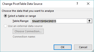
Figure 1. The Change PivotTable Data Source dialog box.

Make sure the cell range in the Table/Range field reflects accurately the range you want included in the PivotTable.

You should note that if you are adding rows in the middle of the PivotTable's data range, or if you delete rows, you do not need to be concerned about the cell range reflected in the Change PivotTable Data Source dialog box. Excel will make sure it is adjusted correctly. (You only need to be concerned when you add rows or columns to the end of the cell range.)

ExcelTips is your source for cost-effective Microsoft Excel training. This tip (10371) applies to Microsoft Excel 2007, 2010, 2013, 2016, 2019, and 2021. You can find a version of this tip for the older menu interface of Excel here: Refreshing PivotTable Data.