Vincent has four kids and ten grandkids. He's in charge of putting together a gift exchange list each Christmas. If he has each of the 14 names in column A (giver), he wonders of there is a formula he can use in column B (recipient) to generate a random name that won't result in someone giving a gift to themselves or being listed as a recipient multiple times.
If you are using the version of Excel in Microsoft 365 or Excel 2021, this task is rather easy, using the RANDARRY and SORTBY functions. Let's assume that you have your names in column A, and that they begin at cell A2. (In cell A1 you have a column title, such as "Giver.") In column B2, place the following formula:
=SORTBY(A2:A15,RANDARRAY(14,1,1,14,TRUE))
The heart of this formula is the RANDARRAY function. It returns an array of random numbers based on the parameters used in the function. The first two parameters (14 and 1) are easy: they represent how many rows and columns of random numbers you want the function to return. In this case, we only need 14 names returned in a single column, thus the parameters used.
The next two parameters indicate the lower and upper values for the range of random numbers. In this case, I chose 1 and 14. This means that RANDARRAY will return 14 values from within the range of 1 to 14. There will be duplicates within this range, but at this point it doesn't really matter.
The final parameter (TRUE) indicates that I want to have integer values in the array. I could have left this out, and it wouldn't really have changed the outcome of the formula, but I find it easier, conceptually, to deal with integers.
The values returned by RANDARRAY are then used to control how the values in cells A2:A15 are sorted. Thus, you end up with 14 random names with no duplicates because there were no duplicates in the source names (A2:A15). There is a possibility, though, that someone will be listed as both the giver and receiver of the same gift. You can add a test for this by placing the following formula in cell C2:
=IF(A2=B2,"Whoa!","")
Copy this down, and you are set. You can regenerate your list by pressing F9, and if the giver and receiver are the same, you'll see "Whoa!" appear in column C. If that occurs, just press F9 again until you don't see anything in the column.
Note that this tip, thus far, applies to Excel in Microsoft 365 and Excel 2021 because only those versions of Excel include the RANDARRAY and SORTBY functions. If you are using a different version of Excel, then you'll need to use a different approach.
Start by making sure you have your column titles set up. In cells A1:G1, enter the values "Giver," "Receiver," "Number," "Rand," "Rank," "Self," and "Unique." Then, make sure that cells A2:A15 contain your 14 different names.
Next, in cells C2:G2, enter the following formulas:
Cell C2: =ROW()
Cell D2: =RAND()
Cell E2: =RANK(D2,$D$2:$D$15)+1
Cell F2: =IF(C2=E2,"Press F9","")
Cell G2: =IF(SUM($C$2:$C$15)=SUM($E$2:$E$15),"","Press F9")
Copy these values down for the rest of the cells, C3:G15. Then, in cell B2, place the following formula:
=OFFSET($A$1,MATCH(E2,$C$2:$C$15,0),0)
Copy it down to cells B3:B15, and you are ready to go. If columns F (Self) and G (Unique) are empty, then you've got a good list in your Receiver column. If you see the text "Press F9" in either column F or G, then do that (press F9) until the columns are empty.
Another possible approach is to use the custom lists feature of Excel. All you need to do is to place the names in the Giver column (A), highlight those names, and then create a custom list that contains those names. Excel allows you to define custom lists very easily, as described in this tip:
https://tips.net/T6243
Once your custom list is defined, select the first Giver name, in cell A2. Then, drag the cell fill handle (small black square at the bottom-right of the cell) to the right. Notice that the names from your custom list are filled out into those cells. Do the same thing for the rest of the names (A3:A15), and what you end up with is giver/recipient list for as many years as you want.
Finally, what tip would be complete without a macro-based approach? If you want to use a macro to generate your list, then the following macro should do the trick just fine:
Sub DoReceivers()
    Dim iKey() As Integer
    Dim iControl() As Integer
    Dim sNames() As String
    Dim maxval As Integer
    Dim iRow As Integer
    Dim iCol As Integer
    Dim j As Integer
    Dim k As Integer
    Dim Ptr As Integer
    Dim c As Range
    Dim s As Range
    Dim sTemp As String
    Dim bGood As Boolean

    Randomize

    Set s = Selection

    If s.Columns.Count > 1 Then
        MsgBox "Please select only cells in a single column"
    Else
        maxval = s.Cells.Count
        iRow = s.Row
        iCol = s.Column

        ReDim iKey(maxval)
        ReDim iControl(maxval)
        ReDim sNames(maxval)

        'Fill the array of values
        j = 0
        For Each c In s
            j = j + 1
            sNames(j) = c.Value
        Next c

        bGood = False
        'Fill the sort key and the control array
        For j = 1 To maxval
            iKey(j) = Int((Rnd * maxval) + 1)
            iControl(j) = iKey(j)
        Next j

        While Not bGood
            'Sort the array based on the random numbers
            For j = 1 To maxval - 1
                Ptr = j
                For k = j + 1 To maxval
                    If iKey(Ptr) > iKey(k) Then Ptr = k
                Next k
                If Ptr <> j Then
                    sTemp = sNames(Ptr)
                    sNames(Ptr) = sNames(j)
                    sNames(j) = sTemp

                    k = iKey(Ptr)
                    iKey(Ptr) = iKey(j)
                    iKey(j) = k
                End If
            Next j

            'Check to see if any Giver/Receiver the same
            bGood = True
            For j = 1 To maxval
                If iKey(j) = iControl(j) Then
                    bGood = False
                    'Fill the sort key and the control array again
                    For k = 1 To maxval
                        iKey(k) = Int((Rnd * maxval) + 1)
                        iControl(k) = iKey(k)
                    Next k
                    Exit For
                End If
            Next j
        Wend

        'Fill in the cells
        For j = 1 To maxval
            Cells(iRow + j - 1, iCol + 1) = sNames(j)
        Next j
    End If
End Sub
Select the range of givers before running the macro. It then grabs all the names and stuffs them in an array. A randomized key array is then set up with a control array being set to the same randomized values. The names are then sorted according to the key array, and then the key array compared to the control array. If any of them are the same (which means that the giver and receiver would be the same, then new random key and control arrays are generated and everything sorted again.
Once a successful sort and giver/receiver check is done, then the receiver names are placed in the cells just to the right of the giver names.
If you want to forego the Excel approach entirely, then you can do a search for phone apps that can handle the task for you. Just search in your preferred app store for "secret santa," and you should have plenty of options.
Note:
ExcelTips is your source for cost-effective Microsoft Excel training. This tip (10418) applies to Microsoft Excel 2007, 2010, 2013, 2016, 2019, 2021, and Excel in Microsoft 365.

Dive Deep into Macros! Make Excel do things you thought were impossible, discover techniques you won't find anywhere else, and create powerful automated reports. Bill Jelen and Tracy Syrstad help you instantly visualize information to make it actionable. You�ll find step-by-step instructions, real-world case studies, and 50 workbooks packed with examples and solutions. Check out Microsoft Excel 2019 VBA and Macros today!
Got a list of data from which you want to delete duplicates? There are a couple of techniques you can use to get rid of ...
Discover MoreIf you want to add up the contents of a range of cells based on what is contained in a different range of cells, you need ...
Discover MoreFormulas are the heart of using Excel, and formulas often refer to ranges of cells. How you insert cells into the ...
Discover MoreFREE SERVICE: Get tips like this every week in ExcelTips, a free productivity newsletter. Enter your address and click "Subscribe."
2024-04-15 14:04:11
Kevin Holliday
I saw this tip after I resolved the same issue. I used ChatGPT and ended up with something similar. You can read about it in this post on LinkedIn.
https://www.linkedin.com/feed/update/urn:li:activity:7185338954496311297/
Thank you, Allen Wyatt.
2024-01-28 10:44:21
J. Woolley
My previous comment below discussed volatile functions in the Tip's solution with RAND, RANK, etc. Its solution with RANDARRAY is also volatile, so the results will probably change each time the workbook is opened or any cell on any worksheet changes (unless you have set Calculation to Manual). Therefore, you might want to copy the RANDARRAY results to a separate column using PASTE VALUES (Alt+H+V+V) to make them non-volatile.
2024-01-28 01:05:23
Tomek
@Ron S:
It is true that (and Allen mentioned it too) there are many solutions available for Secret Santa. However, they may or may not give you exactly what you want, and figuring out how to do it yourself within Excel may come handy for some other task you want to do.
2024-01-28 00:36:00
Tomek
I propose a slightly different macro approach, combining ideas from the firs approach with much simpler macro than proposed.
Assuming giver names are in column A starting in row 2, and recipient names will be generated in column B starting with cell B2. For 14 names this will the be ranges A2:A15 and B2:B15, respectively. For different number of names adjust the formulas and ranges in the macro accordingly.
Create two helper columns. In column C there will be random numbers by which the names will be sorted for column C. These random numbers will be placed there by a macro, but as explicit numbers, so they will not change unless the macro is re-run.
In cell B2 enter the formula =SORTBY(A2:A15,C2:C15). Similarly to what was suggested in the tip, this will sort the names based on random numbers that will be in column C. As at the beginning there are no numbers in column C, the column B will just have the same order as column A, until a macro is run.
In column D in cell D2 enter =B2=A2. Copy this formula down for as many row as there are names. In cell D1 enter formula =OR(D2:D14). This cell will evaluate to TRUE if any giver would be the receiver of their own gift. This will trigger the macro to loop until such situation is resolved.
(see Figure 1 below) for a screenshot of the worksheet.
Now, here is the macro; you can assign it to QAT, a keyboard shortcut, or best, to a button on the spreadsheet:
------------------------
Sub populate()
Dim cel As Range
Randomize
Do
For Each cel In Range("C2:C15")
cel.Value = Rnd()
Next
Loop Until Range("D1").Value = False
End Sub
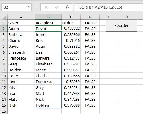
Figure 1.
2024-01-27 14:20:28
J. Woolley
The Tip's solution with RAND, RANK, OFFSET, and MATCH has a small problem. Some of those functions are volatile; therefore, the results will probably change each time the workbook is opened or the worksheet is activated (unless you have set Calculation to Manual). To solve the problem:
1. Follow all of the Tip's instructions to complete cells A1:G15.
2. Change the heading in cell B1 from "Receiver" to "Trial."
3. Insert a column between A and B, which should move columns B:G into C:H.
4. "Trial" should now be in cell C1. Enter "Receiver" in the new cell B1.
5. Press F9 until columns labeled "Self" and "Unique" are blank.
6. Copy results under "Trial" (cells C2:C15) and PASTE VALUES (Alt+H+V+V) under "Receiver" (cells B2:B15); these final results will not change.
To generate new results, repeat steps 5 and 6.
2024-01-27 06:55:58
Ron S
If you don't want to learn how to do the formulas, or want to look at an example that you can analyze, the simple answer is "google is your friend". Search the web for a free template that you can download! There are LOTS.
Like so many "problems" in Excel, the answer is to Reframe your question.
What you describe is commonly known as a "Secret Santa" list. There are lots of sites that provide templates you can download to do this for you.
Got a version of Excel that uses the ribbon interface (Excel 2007 or later)? This site is for you! If you use an earlier version of Excel, visit our ExcelTips site focusing on the menu interface.
FREE SERVICE: Get tips like this every week in ExcelTips, a free productivity newsletter. Enter your address and click "Subscribe."
Copyright © 2026 Sharon Parq Associates, Inc.
Comments