Controlling Data Entry in a Cell

Murray needs a way to control the entry of data into cell B1. If cell A1 contains the capital letter "A," then the user should be able to enter data into cell B1. If cell A1 contains anything but the capital letter "A," then no data entry should be allowed in cell B1 and cell B1 should show "N/A" (not the error value #N/A, but the letters "N/A").

There are two ways to go about this. One way is to use a macro that checks to see if A1 contains "A" or not. If it does, then the macro keeps whatever is in cell B1, unless B1 had previously been set to "N/A." (If it had, then B1 is cleared.) If A1 does not contain "A," then whatever is in cell B1 is replaced with the characters "N/A."

Private Sub Worksheet_Change(ByVal Target As Range)
    Dim sTemp As String

    If Target.Address(False, False) = "A1" Or _
      Target.Address(False, False_ = "B1" Then

        'Store B1's text in variable
        sTemp = Range("B1").Text

        Application.EnableEvents = False
        If Range("A1").Text = "A" Then
            If sTemp = "N/A" Then Range("B1") = ""
        Else
            Range("B1") = "N/A"
        End If
        Application.EnableEvents = True
    End If
End Sub

Note that this is simply one macro-based approach; there are many other approaches that could be used, depending on what behavior you want to have take place if either cell A1 or B1 are selected. In the case of this macro, it should be saved in the ThisWorkbook module so that it triggers whenever something is changed in the worksheet.

The other approach you can use doesn't involve macros at all. Instead, it relies on conditional formatting. Follow these steps:

1. Select cell B1.
2. With the Home tab of the ribbon displayed, click the Conditional Formatting option in the Styles group. Excel displays a palette of options related to conditional formatting.
3. Click Manage Rules. Excel displays the Conditional Formatting Rules Manager dialog box.
4. Click New Rule. Excel displays the New Formatting Rule dialog box.
5. In the Select a Rule Type area at the top of the dialog box, choose Use a Formula to Determine Which Cells to Format. (In Excel 2013 and Excel 2016, click on New Rule and then select Use a Formula to Determine Which Cells to Format.) (See Figure 1.)



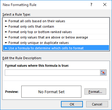
Figure 1. The New Formatting Rule dialog box.

6. In the Format Values Where This Formula Is True box, enter the following: =NOT(EXACT(LEFT(A1,1),"A")). This formula will return True if the cell contains do not contain the letter "A" as the first letter of the cell.
7. Click Format to display the Format Cells dialog box.
8. In the Category list, choose Custom.
9. In the Type box, enter this: "N/A";"N/A";"N/A";"N/A" (make sure you include the quote marks, as shown).
10. Click OK to dismiss the Format Cells dialog box. The formatting you specified in step 7 should now appear in the preview area for the rule.
11. Click OK. The New Formatting Rule dialog box disappears and Excel again displays the Conditional Formatting Rules Manager dialog box. The rule you just defined is listed in the dialog box.
12. Click OK. Excel applies the conditional formatting to cell B1.

The custom format you defined in step 9 causes Excel to display the letters "N/A" when the value is a number (positive, negative, or zero) or text. Since you set all 4 conditions to the same thing, then all of them will display "N/A." This approach changes the display, but it still allows the user to enter a value into cell B1—it just won't display properly unless the first letter in cell A1 is "A."

ExcelTips is your source for cost-effective Microsoft Excel training. This tip (13457) applies to Microsoft Excel 2007, 2010, 2013, 2016, 2019, Excel in Microsoft 365, and 2021.