Written by Allen Wyatt (last updated March 1, 2025)
This tip applies to Excel 2007, 2010, 2013, 2016, 2019, 2021, 2024, and Excel in Microsoft 365
Kris knows how to filter information in a worksheet by color. The filtering tools allow him to select which color of text or background he wants to display. Kris wonders if there is a way to filter so that multiple colors are displayed. If he is filtering by cell contents, he can easily pick multiple matching items to be displayed but cannot figure out how to do it for colors.
There are two ways you can go about this. The first approach doesn't rely on filtering at all. Instead, sort your data by color. If you do two (or more) sorting passes, you should be able to get the desired colors all next to each other. Then, select the remaining rows (the one using colors you don't want to see) and hide those rows.
Again, this is just a workaround, and it can work fine for relatively short lists of data. The second approach is to use a helper column. All you need to do is to enter, in each cell of the helper column, the name of the color in that row—i.e., red, orange, yellow, green, etc. You can then filter by that column and thereby display multiple colors in your filtered results.
If your data table is too long, typing all those colors could get monotonous and be prone to errors. You could, if desired, create two very short user-defined functions that would simply return the color of a specific cell. This UDF returns the color of the text itself:
Function FColor(cell)
    FColor = cell.Font.ColorIndex
End Function
The following is a variation that returns the interior color of the cell itself:
Function IColor(cell)
    IColor = cell.Interior.ColorIndex
End Function
In your helper column, enter a formula that relies on the desired UDF. For instance, if you want to filter by the interior color in column A, you would enter this formula in the helper column of row 1:
=IColor(A1)
The cell should now contain the color number. Copy this cell down as far as necessary, and then filter by the contents of this column. Since you can select multiple numeric values to appear in your filtered data, you effectively end up with multiple colors in the results.
Note:
ExcelTips is your source for cost-effective Microsoft Excel training. This tip (13611) applies to Microsoft Excel 2007, 2010, 2013, 2016, 2019, 2021, 2024, and Excel in Microsoft 365.

Best-Selling VBA Tutorial for Beginners Take your Excel knowledge to the next level. With a little background in VBA programming, you can go well beyond basic spreadsheets and functions. Use macros to reduce errors, save time, and integrate with other Microsoft applications. Fully updated for the latest version of Office 365. Check out Microsoft 365 Excel VBA Programming For Dummies today!
If you have a lot of data in a worksheet, you may want to filter it to display rows that match a particular criterion. ...
Discover MoreThe filtering capabilities of Excel can come in handy for zeroing in on the data you want to work with. When your data ...
Discover MoreFiltering is a great asset when you need to get a handle on a subset of your data. Excel even makes it easy to copy the ...
Discover MoreFREE SERVICE: Get tips like this every week in ExcelTips, a free productivity newsletter. Enter your address and click "Subscribe."
2025-03-11 13:46:19
J. Woolley
Both of the Tip's functions return a ColorIndex property's value. ColorIndex picks from the 56 color current palette, which is usually the same as the default palette. The first 2 colors are black and white, leaving 54 actual colors. But 10 colors in the default palette are duplicates, so only 44 of the 54 are unique. A broader range of colors is given by the Color property, which is a combination of red, green, and blue values (RGB).
The AboutColors macro in My Excel Toolbox creates a worksheet illustrating all colors defined by Excel: Current Palette, Default Palette, Theme Color, Standard Color, vbColor, vbSystemColor, and xlRgbColor. Notice two different Color values might be represented by the same ColorIndex value (see Figure 1 below) .
Here are My Excel Toolbox alternatives to the Tip's FColor and IColor functions, where ColorRGB is equivalent to RGB Long:
=FontColor([Cell]) -- returns Cell's font ColorRGB
=FillColor([Cell]) -- returns Cell's interior fill ColorRGB
Both of these functions return "conditional" if the cell has a conditional format specifying a color different from the base color, even if the condition is not satisfied.
The following functions are also included in My Excel Toolbox:
=ColorRGB(R, G, B)
=ColorName(ColorRGB)
=ColorIndex_Name(ColorIndex)
=ColorAsRed(ColorRGB)
=ColorAsGreen(ColorRGB)
=ColorAsBlue(ColorRGB)
=ColorAsHex(ColorRGB)
=HexAsColor(HexRGB)
=Darkness(ColorRGB)
=IsCurrentPalette(ColorRGB)
=IsDefaultPalette(ColorRGB)
=SetFill([Color], [PatternStyle], [PatternColor], [Target])
=SetFont([Name], [Size], [Style], [Color], [Underline], ..., [Target])
=ChooseColor_Dialog(DefaultColor, CustomColors())
=CurrentPalette() -- returns an array of ColorRGB values
=DefaultPalette() -- returns an array of ColorRGB values
=ThemeColors() -- returns an array of ColorRGB values
=StandardColors() -- returns an array of ColorRGB values
See https://sites.google.com/view/MyExcelToolbox/
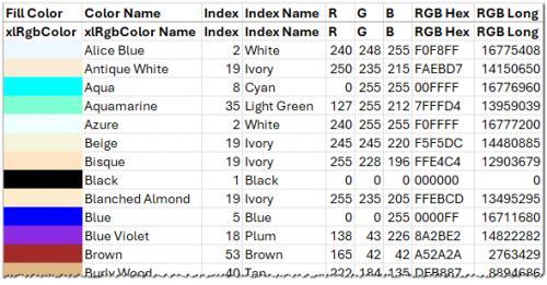
Figure 1.
Got a version of Excel that uses the ribbon interface (Excel 2007 or later)? This site is for you! If you use an earlier version of Excel, visit our ExcelTips site focusing on the menu interface.
FREE SERVICE: Get tips like this every week in ExcelTips, a free productivity newsletter. Enter your address and click "Subscribe."
Copyright © 2025 Sharon Parq Associates, Inc.
Comments