Printing Individual Worksheets for Vendors

Mitchell has a lot of data in a worksheet that represents all of his company's purchase orders for a year. The data is sorted on column C, which contains the vendors' names. Mitchell wants to print a separate page for each vendor with all the data for those rows. He wonders if there is any way to automate the printing of vendor-specific sheets.

As with many things in Excel, there are multiple approaches you can take for this problem. I'm going to look at four approaches in this tip. All four approaches assume that your data is sorted according to the vendor-name column (column C) and that you have column heads on each column of your data (Name, Date, PO Number, Vendor, etc.).

Using Subtotals

To print vendor-specific sheets using subtotals, start by selecting a cell within your data. (A cell in column C would be perfect.) If your data is non-contiguous, you may need to select all of it manually; if it is contiguous, however, then selecting the single cell should be sufficient. Then, follow these steps:

1. Display the Data tab of the ribbon.
2. In the Outline group click the Subtotal tool. Excel displays the Subtotal dialog box. (See Figure 1.)



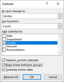
Figure 1. Specifying how subtotals should be created.

3. Make sure the At Each Change In drop-down list is set to Vendor. (Use the name of column C.) This indicates where Excel will insert subtotals.
4. The Use Function drop-down list should be set to Count.
5. Using the list in the Add Subtotal To box, select the Vendor (column C) column. This is where the count will be added.
6. Make sure the check box for Replace Current Subtotals is selected.
7. Make sure the Page Breaks between Groups check box is selected.
8. Make sure the Summary Below Data check box is selected.
9. Click on OK.

Excel places subtotals in your worksheet, but it should also place page breaks before each new vendor. (This is because of step 7, above.) The page breaks may not be immediately obvious, but they come into play when you print the worksheet.

Once printed, what you end up with is a printed page for each of your vendors. The subtotal just below the last row on each page indicates the number of purchase orders printed for that particular vendor.

Using Filtered Data

Filtering your data is quite easy, and this is a good approach if you don't need to print these types of reports that often. Again, start by selecting a cell within your data, unless your data is non-contiguous. (In that case you'll need to manually select all your data.) Then, follow these steps:

1. Display the Data tab of the ribbon.
2. Click the Filter tool within the Sort & Filter group. Excel should display the AutoFilter drop-down indicators next to each column label in row 1.
3. Using the drop-down indicator for the Vendor column (column C), choose the name of the vendor you want to print. Your list is automatically filtered to only display purchase orders from that vendor.
4. Print the page as you normally would. The printed report should show only purchase orders for the vendor you specified in step 3.

If you want to print reports for other vendors, all you need to do is to change the filter (step 3) and reprint (step 4). When you are done, you can remove the filter by again clicking the Filter tool on the Data tab of the ribbon.

Using PivotTables

Another fast way to create the reports you want is to use the PivotTable capabilities of Excel. I won't go into how to create a PivotTable here, as that has been covered in other issues of ExcelTips. Your PivotTable can be set up just about any way you desire, but you need to make sure that the Vendor field is in the Filters group of the PivotTable Fields pane. (See Figure 2.)

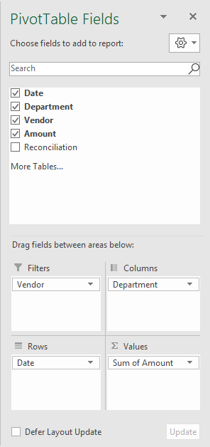
Figure 2. Setting up your PivotTable.

Next, display either the Options or Analyze tab of the ribbon, depending on your version of Excel. (These tabs are only visible when you select a cell within your PivotTable.) In the PivotTable group, at the left of the ribbon, click the Options drop-down list and choose Show Report Filter Pages. (This option is available only if you made sure that the Vendor field is in the Filters group, as mentioned earlier.) Excel displays the Show Report Filter Pages dialog box. (See Figure 3.)

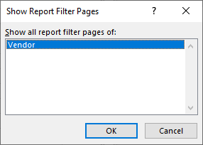
Figure 3. The Show Report Filter Pages dialog box.

There should be only a single field listed in the dialog box, unless you added more than the Vendor field to the Filters group. If there is more than one field listed, make sure you click on the Vendor field. When you click on OK, Excel creates separate PivotTable worksheets for each vendor in your data table. Depending on the information you chose to include in the PivotTable, these can make great reports for your vendors. You can then print the worksheets to get the reports you want.

Using Macros

There are many ways that you could set up a macro to give you the data you want. Personally, I prefer a macro that will go through your data and create new worksheets for each vendor. That's what the following macro does—it compiles a list of vendors from your data and then creates a worksheet named for each vendor. It then copies information from the original worksheet to the newly created worksheets.

Sub CreateVendorSheets()
    ' To use this macro, select the first cell in
    ' the column that contains the vendor names.

    Dim sTemp As String
    Dim sVendors(99) As String
    Dim iVendorCounts(99) As Integer
    Dim iVendors As Integer
    Dim rVendorRange As Range
    Dim c As Range
    Dim J As Integer
    Dim bFound As Boolean

    ' Find last row in the worksheet
    Set rVendorRange = ActiveSheet.Range(Selection, _
      ActiveSheet.Cells(Selection.SpecialCells(xlCellTypeLastCell).Row, _
      Selection.Column))

    ' Collecting all the vendor names in use
    iVendors = 0

    For Each c In rVendorRange
        bFound = False
        sTemp = Trim(c)
        If sTemp > "" Then
            For J = 1 To iVendors
                If sTemp = sVendors(J) Then bFound = True
            Next J
            If Not bFound Then
                iVendors = iVendors + 1
                sVendors(iVendors) = sTemp
                iVendorCounts(iVendors) = 0
            End If
        End If
    Next c

    ' Create worksheets
    For J = 1 To iVendors
        Worksheets.Add After:=Worksheets(Worksheets.Count)
        ActiveSheet.Name = sVendors(J)
    Next J

    ' Start copying information
    Application.ScreenUpdating = False
    For Each c In rVendorRange
        sTemp = Trim(c)
        If sTemp > "" Then
            For J = 1 To iVendors
                If sTemp = sVendors(J) Then
                    iVendorCounts(J) = iVendorCounts(J) + 1
                    c.EntireRow.Copy Sheets(sVendors(J)). _
                      Cells(iVendorCounts(J), 1)
                End If
            Next J
        End If
    Next c
    Application.ScreenUpdating = True
End Sub

As noted at the beginning of the macro, you should select the first cell of data in the Vendor column before running the macro. When completed, you'll have one worksheet for each vendor, which you can format and print as desired. (You could make the macro even more useful by adding code that will put column heading information or other information into each created worksheet.) When done, you'll need to delete the worksheets for those vendors so that the next time you run the macro you don't run into a problem.

ExcelTips is your source for cost-effective Microsoft Excel training. This tip (13633) applies to Microsoft Excel 2007, 2010, 2013, 2016, 2019, 2021, 2024, and Excel in Microsoft 365.