Please Note: This article is written for users of the following Microsoft Excel versions: 2007, 2010, 2013, 2016, 2019, and 2021. If you are using an earlier version (Excel 2003 or earlier), this tip may not work for you. For a version of this tip written specifically for earlier versions of Excel, click here: Locking Callouts to a Graph Location.
After creating a chart in Excel, you may want to add a callout or two to the chart. For instance, there may be a spike or an anomaly in the data, and you want to include a callout that explains the aberration.
Callouts, when drawn using the drawing tools available in Excel, are graphic objects that have a "connector" that can point where you want it. This makes them great for pointing to the aberration you want explained in your chart. The problem is, if you change the data range displayed in the chart, the perspective of the chart changes, and the callout no longer points to where it used to point. (It still points to where the aberration used to appear on the chart.)
The reason for this is that the callout and the chart are not related. The callout isn't locked to a specific place on the chart; it just overlays the chart to give the desired effect. There is no way in Excel to link a callout to a specific chart point.
Most people use a different approach to adding explanatory text to their charts. Instead of using a callout, they use data labels to achieve the same purpose. Follow these steps:
You can also format the data label's font and color, as desired, and you can move the data label's position by dragging it to a different area. The data label will maintain the same relative position to the data point, even when the chart is changed.
ExcelTips is your source for cost-effective Microsoft Excel training. This tip (1154) applies to Microsoft Excel 2007, 2010, 2013, 2016, 2019, and 2021. You can find a version of this tip for the older menu interface of Excel here: Locking Callouts to a Graph Location.

Program Successfully in Excel! This guide will provide you with all the information you need to automate any task in Excel and save time and effort. Learn how to extend Excel's functionality with VBA to create solutions not possible with the standard features. Includes latest information for Excel 2024 and Microsoft 365. Check out Mastering Excel VBA Programming today!
As components of the Microsoft Office suite, one would expect Excel and Word to work together. One of the most common ...
Discover MoreYou can create hyperlinks to all sorts of worksheets in a workbook, but you cannot create a hyperlink to a chart sheet. ...
Discover MoreIf the data you are using as the source for a chart includes some cells that are empty, you may want to exclude those ...
Discover MoreFREE SERVICE: Get tips like this every week in ExcelTips, a free productivity newsletter. Enter your address and click "Subscribe."
2020-12-19 11:30:53
Pat Little
This tip works as stated - I can add a data label (callout) for a single data point and use a formula to display the label text from a cell of my choice. After saving and re-opening the file it shows the same one label I created.
However, if I want to use Excel's built-in way of adding labels using cell values (I'm using Office Standard 2019) then I have problems. My first image shows what Excel displays after I set up data labels using cell values in col C
(see Figure 1 below)
which is just what I want - it shows labels for the data points where I have something in col C and no labels for all the other data points.
BUT - when I save the workbook and re-open it Excel has added labels for EVERY data point not just those where I have something in col C. As shown below:
(see Figure 2 below)
Am I doing something wrong, or is this just the way that Excel works? If the latter then it seems like a bug.
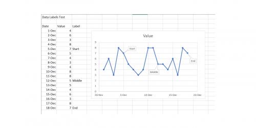
Figure 1. Add data labels from cell values but before save the file
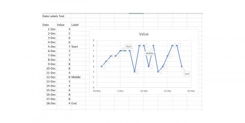
Figure 2. After save and re-open the file
2020-04-13 11:54:20
Hi- I have been using this method for quite some time. I think I just ran into a bug though. I had a set of labels on specific data points, just as you describe above, but recently, sometime after appending new data (my x-axis is date/time), and my chart grows to the right as typical, my data labels are now assigned to different points altogether. I cannot think of any other change that was made to my spreadsheet, no deletion of data, rows, etc. I have scoured the internet for clues on this by am not finding anything. Do you have any ideas? I had thought this might be a reliable way to have a record and display of anomalous events, but now think I am back to the drawing board.
2017-03-16 12:22:51
Daniel Reddy
Is there a way to make the data callout shift over to the latest data point as you add new data?
2016-05-20 03:38:10
Nev
Excellent tip! I knew there must be a way to do this, but couldn't discover it unaided. Thanks.
2015-07-26 09:51:01
ALan
In my Excel 2010, I tried to use a call reference such as =F7 in step 4.
I got an error message "References in series formulas must be external references to worksheets" and had to use =name!$F$7 instead (where 'name' is the worksheet name).
2015-07-11 22:09:32
Bob Beechey
Instead of Add Data Label, you can also use Add Data Callout in Excel 2013
Got a version of Excel that uses the ribbon interface (Excel 2007 or later)? This site is for you! If you use an earlier version of Excel, visit our ExcelTips site focusing on the menu interface.
FREE SERVICE: Get tips like this every week in ExcelTips, a free productivity newsletter. Enter your address and click "Subscribe."
Copyright © 2026 Sharon Parq Associates, Inc.
 Please Note:
This article is written for users of the following Microsoft Excel versions: 2007, 2010, 2013, 2016, 2019, and 2021. If you are using an earlier version (Excel 2003 or earlier), this tip may not work for you. For a version of this tip written specifically for earlier versions of Excel, click here:
Please Note:
This article is written for users of the following Microsoft Excel versions: 2007, 2010, 2013, 2016, 2019, and 2021. If you are using an earlier version (Excel 2003 or earlier), this tip may not work for you. For a version of this tip written specifically for earlier versions of Excel, click here:
Comments