Please Note: This article is written for users of the following Microsoft Excel versions: 2007, 2010, 2013, 2016, 2019, and Excel in Microsoft 365. If you are using an earlier version (Excel 2003 or earlier), this tip may not work for you. For a version of this tip written specifically for earlier versions of Excel, click here: Automatic Lines for Dividing Lists.

Automatic Lines for Dividing Lists

Written by Allen Wyatt (last updated December 29, 2022)
This tip applies to Excel 2007, 2010, 2013, 2016, 2019, and Excel in Microsoft 365


5

Let's say you have a list of company transactions. Each transaction includes a department number, a title, and other information (amount, date, authorizer, etc.). As you get more and more of these items in your list, you may want a way to automatically add "dividing lines" based on the department number. For instance, when the department number changes, you may want to include a line between the two departments.

To add this type of formatting to your list, start by sorting your data table by department. For the sake of this example, I'll assume that your data is actually in columns A:F, with the department numbers in column A. (See Figure 1.)

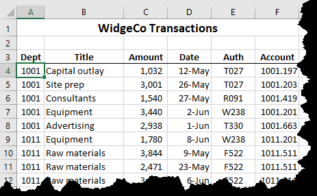
Figure 1. The data to be divided.

To add the automatic dividing lines, follow these steps:

  1. Select the left-most cell of the first row of your data. For instance, if your table heads are in row 3 and your first row of data is in row 4, you should select cell A4.
  2. Press Shift+Ctrl+End. All the cells in your data table should be selected, with the exception of the header row.
  3. With the Home tab of the ribbon displayed, click the Conditional Formatting option in the Styles group. Excel displays a palette of options related to conditional formatting.
  4. Click New Rule. Excel displays the New Formatting Rule dialog box.
  5. In the Select a Rule Type area at the top of the dialog box, choose Use a Formula to Determine Which Cells to Format. (See Figure 2.)
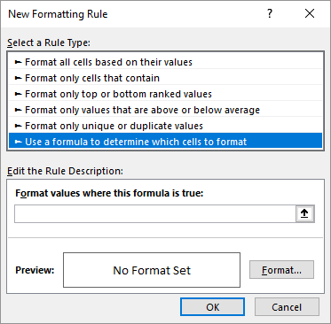
  6. Figure 2. The New Formatting Rule dialog box.

  7. In the Format Values Where This Formula Is True box, enter "=$A4<>$A5" (without the quote marks). This formula, of course, will vary depending on your data. As entered here, it is appropriate for the data table already described in this tip and the cell selected in step 1.
  8. Click Format to display the Format Cells dialog box.
  9. Display the Border tab.
  10. Click the None button to remove any borders already applied to the cells.
  11. In the Style list, select the type of border you want to appear between departments.
  12. In the Border area of the dialog box, click the button that adds your selected border style to the bottom of the cells.
  13. Click OK to dismiss the Format Cells dialog box. The formatting you specified in steps 10 and 11 should now appear in the preview area for the rule.
  14. Click OK.

That's it; you should now see a line that appears across the entire width of your data every time the department changes.

ExcelTips is your source for cost-effective Microsoft Excel training. This tip (6863) applies to Microsoft Excel 2007, 2010, 2013, 2016, 2019, and Excel in Microsoft 365. You can find a version of this tip for the older menu interface of Excel here: Automatic Lines for Dividing Lists.

Author Bio

Allen Wyatt

With more than 50 non-fiction books and numerous magazine articles to his credit, Allen Wyatt is an internationally recognized author. He is president of Sharon Parq Associates, a computer and publishing services company. ...

MORE FROM ALLEN

Measurement of Choice Isn't Persistent

Normally, Word allows you to specify what measurement units you want used for the program; just choose Tools | Options | ...

Discover More

Uncovering and Removing Links

Excel allows you to reference data in other workbooks by establishing links to that data. If you later want to get rid of ...

Discover More

Turning E-mail Addresses into Hyperlinks

Got a whole bunch of e-mail addresses that you need to convert to active hyperlinks? You can do the conversion in a ...

Discover More

Excel Smarts for Beginners! Featuring the friendly and trusted For Dummies style, this popular guide shows beginners how to get up and running with Excel while also helping more experienced users get comfortable with the newest features. Check out Excel 2013 For Dummies today!

More ExcelTips (ribbon)

Shading Based on Odds and Evens

You can use conditional formatting to add shading to various cells in your worksheet. This tip shows how you can shade ...

Discover More

Conditional Formats for Odd and Even Columns

Setting up conditional formatting can be challenging under some circumstances, but once set it can work great. Unless, of ...

Discover More

Finding Cells that Use Conditional Formatting

Conditional Formatting is a great boon to effectively displaying the information in your worksheets. If you want to ...

Discover More
Subscribe

FREE SERVICE: Get tips like this every week in ExcelTips, a free productivity newsletter. Enter your address and click "Subscribe."

View most recent newsletter.

Comments

If you would like to add an image to your comment (not an avatar, but an image to help in making the point of your comment), include the characters [{fig}] (all 7 characters, in the sequence shown) in your comment text. You’ll be prompted to upload your image when you submit the comment. Maximum image size is 6Mpixels. Images larger than 600px wide or 1000px tall will be reduced. Up to three images may be included in a comment. All images are subject to review. Commenting privileges may be curtailed if inappropriate images are posted.

What is nine minus 5?

2019-09-12 21:00:33

Artamov

This was a great tip! I found a macro to do the same, but it wouldn't underline the entire row. TIP: it's written down above, but is easy to miss: DO NOT SELECT THE HEADER ROW! Let's assume the header is Row 1. If you don't select the header row, your formula is "=$a2<>$a3. HOWEVER: If you do select the header row, then either change the "Applies to" in the rule to "=$2:$xxxxxxx", OR change the formula to "=$a1<>$a2".


2019-06-19 03:00:43

SteveJez

BBN,
Assuming your dates are in column A starting in A1 with a title, use the following formula in Conditional Formatting, applied to range A2:?? (to suit your data) & set whatever formatting you want.

=IFERROR(MONTH(A2)<>MONTH(A1),1)

This will find the beginning of the month, if you prefer the end of the month use the following formula applied to the same range

=(MONTH(A3)<>MONTH(A2)

The IFERROR in the first formula deals with the title in A1, it is not required in the second formula as there is no reference to A1.

All the usual warnings when applying Conditional Formatting, as to inserting rows or adding data to the end of the list. It is also possible to use VBA to apply formatting to a required range, but that might be a step too far at the moment.

HTH

Steve


2019-06-18 06:27:00

Richard

Geoff: One option is to apply the conditional formatting way beyond the end of your data. In Home > Conditional Formatting > Manage Rules, adjust the Applies To range to apply the formatting to some suitable row number depending on your data (say row 10,000), e.g. $A$2:$A$10000.
If this produces undesirable effects below your data, qualify the condition using an IF expression, e.g. IF (A2<>"", <your condition>).


2019-06-10 11:34:36

BBN

I used to work for a company that had several hundred clients, for each of which I'd have to perform an annual task on a day specific to that client. I did up a spreadsheet and just manually kept a solid black line between each of the months as I liked to see what was coming up as each month approached. Is there a variation on that formula that could be used on such a spreadsheet to separate the months? (Note: I know I *could* use conditional formatting to just use, example, shading, but two problems: one, I actually dislike shaded cells and find they make data *more* difficult for me to read rather than less. And two, we only had a very old b&w printer, and any spreadsheet using colored cells just looked like garbage when printed off.)


2019-06-08 06:03:40

Geoff Robb

I use this conditional formatting in a spreadsheet I have developed, but I often find that the formatting does not copy down prperly when adding data at the bottom of the table (ie adding rows at the bottom) . Is there a reliable way to have the formatting copied down automatically as new data is entered? I have tried copying the formatting down below the data, but the new rows appear to overwrite the conditional formatting.


This Site

Got a version of Excel that uses the ribbon interface (Excel 2007 or later)? This site is for you! If you use an earlier version of Excel, visit our ExcelTips site focusing on the menu interface.

Newest Tips
Subscribe

FREE SERVICE: Get tips like this every week in ExcelTips, a free productivity newsletter. Enter your address and click "Subscribe."

(Your e-mail address is not shared with anyone, ever.)

View the most recent newsletter.