Missing PivotTable Data

Imagine this scenario—you are working with an Excel workbook created by someone else. The workbook contains a PivotTable, but you discover that you cannot make changes to it. When you try, you get a message that says the underlying data was not saved. The worksheet with the data is in the workbook, and the PivotTable is there, but you cannot change the PivotTable directly or even make changes to the worksheet and updated the PivotTable.

This scenario isn't that unique; it happens all the time. There are two possible reasons for the problem. First, when a PivotTable is created, the user can specify an option that causes Excel to not save the data with the table layout. (This option is accessed by clicking the Options button on the last step of the PivotTable Wizard.) If the PivotTable is really based on the worksheet in the workbook, then this is no problem. If, however, it is based on some other data source, then it can cause a problem because you cannot later modify the table.

The second possible reason is that the workbook that you have isn't the same workbook in which the worksheet and the PivotTable originally resided. It is possible that, in creating the workbook for your use, the original user copied the PivotTable and the worksheet from the original workbook to a new, blank workbook. If this is the case, then the PivotTable is independent of any data in the workbook you are viewing. You can check this out by trying these steps:

1. Click anywhere within the PivotTable.
2. Display the Options tab of the Ribbon (Excel 2007 or Excel 2010. If you are using Excel 2013 or a later version, display the Analyze tab of the Ribbon.)
3. Click the Change Data Source tool in the Data group. Excel displays the Change PivotTable Data Source dialog box. (See Figure 1.)



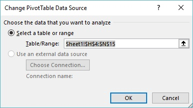
Figure 1. The Change PivotTable Data Source dialog box.

4. In the Table/Range box, specify an address range within the current workbook, specifically within the worksheet data you want to use.
5. Click OK.

Excel redoes the PivotTable, this time based on the information in the workbook. You can then make changes to the PivotTable (or the underlying data) as you desire.

ExcelTips is your source for cost-effective Microsoft Excel training. This tip (8391) applies to Microsoft Excel 2007, 2010, 2013, 2016, 2019, and Excel in Microsoft 365. You can find a version of this tip for the older menu interface of Excel here: Missing PivotTable Data.