Printing Just the Visible Data

It is easy to amass quite a bit of information in an Excel workbook. Fortunately, that information can be easily printed out. What if you only want to print just what you see on the screen, however, instead of an entire worksheet? To make matters worse, what if you are using frozen panes to hold the position of your page headers?

Normally, you could simply choose what you want printed and then just print that selection. Alternately, you could choose what you want printed, define it as the print area, and then choose to print. This simple of an approach won't work in this instance, however, because of using frozen panes. This feature allows you to "freeze" rows at the top of the screen, columns at the left of the screen, and only scroll the cells in the unfrozen part. Thus, you can't select everything you want to print because what you want to print consists of three distinct areas of the worksheet.

The solution is to set Excel's repeating rows and columns, and then choose what you want to print. The following steps work just fine:

1. Display the Page Layout tab of the ribbon.
2. Click the small icon at the lower-right corner of the Page Setup group. Excel displays the Page Setup dialog box.
3. Make sure the Sheet tab is selected. (See Figure 1.)



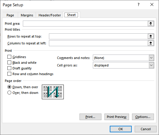
Figure 1. The Sheet tab of the Page Setup dialog box.

4. Place the insertion point in the Rows to Repeat at Top box.
5. In the worksheet, select the rows you want to appear at the top of each page. The row names should appear in the dialog box.
6. Place the insertion point in the Columns to Repeat at Left box.
7. In the worksheet, select the columns you want to appear at the left of each page. The column names should appear in the dialog box.
8. Click on OK to close the Page Setup dialog box.
9. Select the range you want to print, but don't include any cells in the rows or columns you specified in steps 5 and 7.

What you do at this point depends on whether you are using Excel 2007 or a later version. If you are using Excel 2007, follow these steps:

1. Press Ctrl+P. Excel displays the Print dialog box. (See Figure 2.)



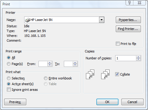
Figure 2. The Print dialog box.

2. Choose the Selection radio button. (You are indicating that you want to print only what you have selected.)
3. Click on OK.

If you are using Excel 2010 or a later version, follow these steps instead:

1. Press Ctrl+P. Excel displays the Print controls on the File tab of the ribbon.
2. Click the first button under the Settings heading and choose Print Selection. (You are indicating that you want to print only what you have selected.)
3. Click on Print.

The printout contains only the cells you specified, along with the frozen rows and columns. If you selected just the visible cells in step 9, then you effectively printed just the visible data.

ExcelTips is your source for cost-effective Microsoft Excel training. This tip (10816) applies to Microsoft Excel 2007, 2010, 2013, 2016, 2019, and 2021. You can find a version of this tip for the older menu interface of Excel here: Printing Just the Visible Data.