Creating a Year-to-Date Comparison Chart

Nora has kept a weather log for years. Each sheet of the workbook is a separate year, with column A on each sheet being the dates in the year and column B being the amount of precipitation on that day, if any. Nora would like to create a chart showing this year's precipitation vs. last year's precipitation, to date. She wonders if there is a way to automatically have this chart reference the correct precipitation values for both years based on today's date.

There are a couple of ways that this need can be filled, depending on exactly what you want to achieve. If you just want to compare rainfall this year to rainfall last year, by date, then you can easily do it by setting up some dynamic named ranges that define the data you want to use.

To begin with, let's assume that your data for 2022 is in a worksheet named 2022 and your data for 2023 (so far) is in a worksheet named 2023. On each worksheet, row 1 contains headings, which means that your dates actually start in cell A2 and your precipitation readings in cell B2. Follow these steps to set up the ranges:

1. Display the Formulas tab of the ribbon.
2. In the Defined Names group, click the Name Manager tool. Excel displays the Name Manager dialog box.
3. Click the New button. Excel displays the New Name dialog box. (See Figure 1.)



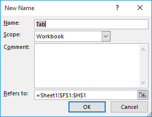
Figure 1. The New Name dialog box.

4. In the Name field, enter the name CurrentYear (note that this is a single word, with no spaces).
5. In the Refers To field, enter the following formula:

=OFFSET(INDIRECT(YEAR(NOW())&"!A1"),1,1,TODAY()-DATE(YEAR(NOW()),1,1)+1,1)

6. Click the OK button to finish creating the named range. The new range should appear in the Name Manager dialog box.
7. Click the New button again. Excel (again) displays the New Name dialog box.
8. In the Name field, enter the name PreviousYear (note that this is, again, a single word, with no spaces).
9. In the Refers To field, enter the following formula:

=OFFSET(INDIRECT(YEAR(NOW())-1&"!A1"),1,1,TODAY()-DATE(YEAR(NOW()),1,1)+1,1)

10. Click the OK button. The new range should appear in the Name Manager dialog box.
11. Click the New button a third time. Excel displays the New Name dialog box.
12. In the Name field, enter the name Dates.
13. In the Refers To field, enter the following formula:

=OFFSET(INDIRECT(YEAR(NOW())&"!A1"),1,0,TODAY()-DATE(YEAR(NOW()),1,1)+1,1)

14. Click the Close button to dismiss the Name Manager dialog box.

With the ranges defined, you can now create the chart using those ranges:

1. Display the Insert tab of the ribbon.
2. In the Charts group click the Column option. Excel displays a drop-down list.
3. Click once on the Clustered Column format. (This is the first option under the 2-D Column heading.) Excel creates a blank chart object in your worksheet.
4. Right-click the chart object. Excel displays a Context menu.
5. Choose Select Data from the Context menu. Excel displays the Select Data Source dialog box, which should be completely empty because you've not added any data ranges to the chart.
6. At the left side of the dialog box, under the Legend Entries (Series) heading, click the Add button. Excel displays the Edit Series dialog box. (See Figure 2.)



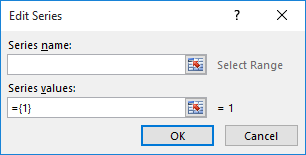
Figure 2. The Edit Series dialog box.

7. In the Series Name field, enter 2022.
8. In the Series Values field, enter this: '2022'!PreviousYear.
9. Click the OK button. The data series now appears in the Select Data Source dialog box.
10. Click, again, the same Add button you clicked in step 6. Excel again displays the Edit Data Series dialog box.
11. In the Series Name field, enter 2023.
12. In the Series Values field, enter this: '2023'!CurrentYear.
13. Click the OK button. This second data series now appears in the Select Data Source dialog box.
14. At the right side of the dialog box, under the Horizontal (Category) Axis Labels heading, click the Edit button. Excel displays the Axis Labels dialog box. (See Figure 3.)



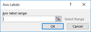
Figure 3. The Axis Labels dialog box.

15. In the Axis Label Range, enter this: '2023'!Dates.
16. Click the OK button. The Select Data Source dialog box should be fully filled out with the necessary information.
17. Click OK to dismiss the Select Data Source dialog box.

Your updated chart, showing only the dates up through today's date, should now be visible. You can continue to format the chart, as desired. (For instance, you'll probably want to format the dates in the chart so they don't include a year.) Further, the chart is dynamic, so that when you open the workbook tomorrow it will reflect one more day than it did today.

Another way to handle it is to reconsider how you are storing your data. Instead of storing all your precipitation readings on separate worksheets (by year), put them all on a single worksheet. Since Excel can handle over a million rows of data in a worksheet, you won't run up against any practical limitations. (A million rows represents well over 2,700 years.)

Now, on a different worksheet, you can use two array formulas to calculate the cumulative rainfall for both years, to date. The following array formula will provide the rainfall for the previous year:

=SUM(Data!B2:B1000*IF(Data!A2:A1000>=DATE(YEAR(NOW())-1,1,1),IF(Data!A2:A1000<=EDATE(NOW(),-12),1,0)))

This assumes that the original precipitation readings are on a worksheet named Data and that they don't extend beyond 1000 rows. (You can modify either of these, as necessary.) To get the to-date rainfall for this year, you can use this array formula:

=SUM(Data!B2:B1000*IF(Data!A2:A1000>=DATE(YEAR(NOW()),1,1),IF(Data!A2:A1000<=NOW(),1,0)))

Remember: These are both array formulas, so they should be entered using Ctrl+Shift+Enter. The single value returned by each formula represents the cumulative rainfall from each year, to date. These two values can then be used in any chart that you want.

ExcelTips is your source for cost-effective Microsoft Excel training. This tip (13427) applies to Microsoft Excel 2007, 2010, 2013, 2016, 2019, Excel in Microsoft 365, and 2021.