Matching Formatting when Concatenating

When using a formula to merge the contents of multiple cells into one cell, Kris is having trouble getting Excel to preserve the formatting of the original cells. For example, assume that cells A1 and B1 contain 1 and 0.33, respectively. In cell C1, he enters the following formula:

=A1 & " : " & B1

The result in cell C1 looks like this:

1:0.3333333333

The reason that the resulting C1 doesn't match what is shown in B1 (0.33) is because the value in B1 isn't really 0.33. Internally, Excel maintains values to 15 digits, so that if cell B1 contains a formula such as =1/3, internally this is maintained as 0.33333333333333. What you see in cell B1, however, depends on how the cell is formatted. In this case, the formatting probably is set to display only two digits beyond the decimal point.

There are several ways you can get the desired results in cell C1, however. One method is to simply modify your formula a bit so that the values pulled from cells A1 and B1 are formatted. For instance, the following example uses the TEXT function to do the formatting:

=TEXT(A1,"0") & " : " & TEXT(B1,"0.00")

In this case, A1 is formatted to display only whole numbers and B1 is formatted to display only two decimal places. You could also use the ROUND function to achieve a similar result:

=ROUND(A1,0) & " : " & ROUND(B1,2)

Another possible solution is to change how Excel deals with precision in the workbook. Follow these steps:

1. Display the Excel Options dialog box. (In Excel 2007 click the Office button and then click Excel Options. In Excel 2010 or a later version, display the File tab of the ribbon and then click Options.)
2. Click the Advanced option at the left of the dialog box.
3. Scroll through the available options until you see the When Calculating This Workbook section. (See Figure 1.)



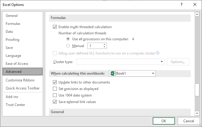
Figure 1. The Advanced options of the Excel Option dialog box.

4. Ensure that the Set Precision As Displayed check box is selected.
5. Click OK.

Now, Excel uses the precision shown on the screen in all of its calculations and concatenations instead of doing calculations at the full 15-digit precision it normally maintains. While this approach may be acceptable for some users, for others it will present more problems than it solves. You will need to determine if you can live with the lower precision in order to get the output formatted the way you expect.

Still another approach is to create your own user-defined function that will return what is displayed for the target cell, rather than what is stored there. The following macro will work great in this regard:

Function FmtText(rng As Range)
    Application.Volatile
    FmtText = rng.Cells(1).Text
End Function

To use this macro, you would use a formula like this in your worksheet:

=FmtText(A1) & " : " & FmtText(B1)

Notice that the function is designated as volatile. This designation means that the macro will run any time that a recalculation is done. This is not strictly necessary, but it is helpful in certain situations. Consider that someone could change the formatting of cell A1. This would not trigger a recalculation, so FmtText will not return an updated text string. However, the next time the recalc is triggered, it will return the re-formatted contents of the cells.

ExcelTips is your source for cost-effective Microsoft Excel training. This tip (8886) applies to Microsoft Excel 2007, 2010, 2013, 2016, 2019, 2021, 2024, and Excel in Microsoft 365. You can find a version of this tip for the older menu interface of Excel here: Matching Formatting when Concatenating.